A lot of people complain that driving across the United States is boring. Having done the coast-to-coast trip seven times now, I can’t agree. Sure, the stretches through the Corn Belt get a little monotonous, but for someone like me who wants to know how everything works, even endless agriculture is fascinating; I love me some center-pivot irrigation.

One thing that has always attracted my attention while on these long road trips is the weigh stations that pop up along the way, particularly when you transition from one state to another. Maybe it’s just getting a chance to look at something other than wheat, but weigh stations are interesting in their own right because of everything that’s going on in these massive roadside plazas. Gone are the days of a simple pull-off with a mechanical scale that was closed far more often than it was open. Today’s weigh stations are critical infrastructure installations that are bristling with sensors to provide a multi-modal insight into the state of the trucks — and drivers — plying our increasingly crowded highways.

All About the Axles

Before diving into the nuts and bolts of weigh stations, it might be helpful to discuss the rationale behind infrastructure whose main function, at least to the casual observer, seems to be making the truck driver’s job even more challenging, not to mention less profitable. We’ve all probably sped by long lines of semi trucks queued up for the scales alongside a highway, pitying the poor drivers and wondering if the whole endeavor is worth the diesel being wasted.

The answer to that question boils down to one word: axles. In the United States, the maximum legal gross vehicle weight (GVW) for a fully loaded semi truck is typically 40 tons, although permits are issued for overweight vehicles. The typical “18-wheeler” will distribute that load over five axles, which means each axle transmits 16,000 pounds of force into the pavement, assuming an even distribution of weight across the length of the vehicle. Studies conducted in the early 1960s revealed that heavier trucks caused more damage to roadways than lighter passenger vehicles, and that the increase in damage is proportional to the fourth power of axle weight. So, keeping a close eye on truck weights is critical to protecting the highways.

Just how much damage trucks can cause to pavement is pretty alarming. Each axle of a truck creates a compression wave as it rolls along the pavement, as much as a few millimeters deep, depending on road construction and loads. The relentless cycle of compression and expansion results in pavement fatigue and cracks, which let water into the interior of the roadway. In cold weather, freeze-thaw cycles exert tremendous forces on the pavement that can tear it apart in short order. The greater the load on the truck, the more stress it puts on the roadway and the faster it wears out.

The other, perhaps more obvious reason to monitor axles passing over a highway is that they’re critical to truck safety. A truck’s axles have to support huge loads in a dynamic environment, and every component mounted to each axle, including springs, brakes, and wheels, is subject to huge forces that can lead to wear and catastrophic failure. Complete failure of an axle isn’t uncommon, and a driver can be completely unaware that a wheel has detached from a trailer and become an unguided missile bouncing down the highway. Regular inspections of the running gear on trucks and trailers are critical to avoiding these potentially catastrophic occurrences.

Ways to Weigh

The first thing you’ll likely notice when driving past one of the approximately 700 official weigh stations lining the US Interstate highway system is how much space they take up. In contrast to the relatively modest weigh stations of the past, modern weigh stations take up a lot of real estate. Most weigh stations are optimized to get the greatest number of trucks processed as quickly as possible, which means constructing multiple lanes of approach to the scale house, along with lanes that can be used by exempt vehicles to bypass inspection, and turnout lanes and parking areas for closer inspection of select vehicles.

In addition to the physical footprint of the weigh station proper, supporting infrastructure can often be seen miles in advance. Fixed signs are usually the first indication that you’re getting near a weigh station, along with electronic signboards that can be changed remotely to indicate if the weigh station is open or closed. Signs give drivers time to figure out if they need to stop at the weigh station, and to begin the process of getting into the proper lane to negotiate the exit. Most weigh stations also have a net of sensors and cameras mounted to poles and overhead structures well before the weigh station exit. These are monitored by officers in the station to spot any trucks that are trying to avoid inspections.

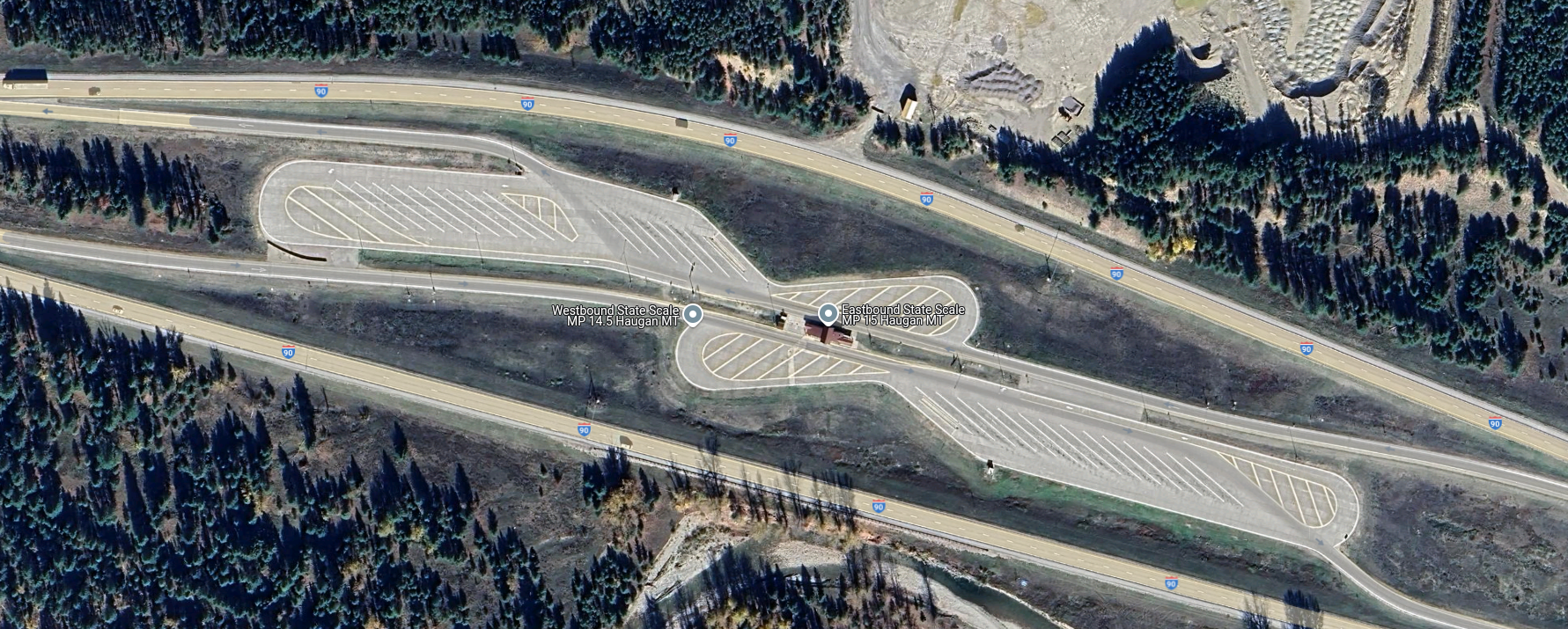
Most weigh stations in the US are located off the right side of the highway, as left-hand exit ramps are generally more dangerous than right exits. Still, a single weigh station located in the median of the highway can serve traffic from both directions, so the extra risk of accidents from exiting the highway to the left is often outweighed by the savings of not having to build two separate facilities. Either way, the main feature of a weigh station is the scale house, a building with large windows that offer a commanding view of the entire plaza as well as an up-close look at the trucks passing over the scales embedded in the pavement directly adjacent to the structure.

Scales at a weigh station are generally of two types: static scales, and weigh-in-motion (WIM) systems. A static scale is a large platform, called a weighbridge, set into a pit in the inspection lane, with the surface flush with the roadway. The platform floats within the pit, supported by a set of cantilevers that transmit the force exerted by the truck to electronic load cells. The signal from the load cells is cleaned up by signal conditioners before going to analog-to-digital converters and being summed and dampened by a scale controller in the scale house.

The weighbridge on a static scale is usually long enough to accommodate an entire semi tractor and trailer, which accurately weighs the entire vehicle in one measurement. The disadvantage is that the entire truck has to come to a complete stop on the weighbridge to take a measurement. Add in the time it takes for the induced motion of the weighbridge to settle, along with the time needed for the driver to make a slow approach to the scale, and each measurement can add up to significant delays for truckers.

To avoid these issues, weigh-in-motion systems are often used. WIM systems use much the same equipment as the weighbridge on a static scale, although they tend to use piezoelectric sensors rather than traditional strain-gauge load cells, and usually have a platform that’s only big enough to have one axle bear on it at a time. A truck using a WIM scale remains in motion while the force exerted by each axle is measured, allowing the controller to come up with a final GVW as well as weights for each axle. While some WIM systems can measure the weight of a vehicle at highway speed, most weigh stations require trucks to keep their speed pretty slow, under five miles per hour. This is obviously for everyone’s safety, and even though the somewhat stately procession of trucks through a WIM can still plug traffic up, keeping trucks from having to come to a complete stop and set their brakes greatly increases weigh station throughput.

Another advantage of WIM systems is that the spacing between axles can be measured. The speed of the truck through the scale can be measured, usually using a pair of inductive loops embedded in the roadway around the WIM sensors. Knowing the vehicle’s speed through the scale allows the scale controller to calculate the distance between axles. Some states strictly regulate the distance between a trailer’s kingpin, which is where it attaches to the tractor, and the trailer’s first axle. Trailers that are not in compliance can be flagged and directed to a parking area to await a service truck to come by to adjust the spacing of the trailer bogie.

Keep It Moving, Buddy

Despite the increased throughput of WIM scales, there are often too many trucks trying to use a weigh station at peak times. To reduce congestion further, some states participate in automatic bypass systems. These systems, generically known as PrePass for the specific brand with the greatest market penetration, use in-cab transponders that are interrogated by transmitters mounted over the roadway well in advance of the weigh station. The transponder code is sent to PrePass for authentication, and if the truck ID comes back to a company that has gone through the PrePass certification process, a signal is sent to the transponder telling the driver to bypass the weigh station. The transponder lights a green LED in this case, which stays lit for about 15 minutes, just in case the driver gets stopped by an overzealous trooper who mistakes the truck for a scofflaw.

PrePass transponders are just one aspect of an entire suite of automatic vehicle identification (AVI) systems used in the typical modern weigh station. Most weigh stations are positively bristling with cameras, some of which are dedicated to automatic license plate recognition. These are integrated into the scale controller system and serve to associate WIM data with a specific truck, so violations can be flagged. They also help with the enforcement of traffic laws, as well as locating human traffickers, an increasingly common problem. Weigh stations also often have laser scanners mounted on bridges over the approach lanes to detect unpermitted oversized loads. Image analysis systems are also used to verify the presence and proper operation of required equipment, such a mirrors, lights, and mudflaps. Some weigh stations also have systems that can interrogate the electronic logging device inside the cab to verify that the driver isn’t in violation of hours of service laws, which dictate how long a driver can be on the road before taking breaks.

Sensors Galore

Another set of sensors often found in the outer reaches of the weigh station plaza is related to the mechanical status of the truck. Infrared cameras are often used to scan for excessive heat being emitted by an axle, often a sign of worn or damaged brakes. The status of a truck’s tires can also be monitored thanks to Tire Anomaly and Classification Systems (TACS), which use in-road sensors that can analyze the contact patch of each tire while the vehicle is in motion. TACS can detect flat tires, over- and under-inflated tires, tires that are completely missing from an axle, or even mismatched tires. Any of these anomalies can cause a tire to quickly wear out and potentially self-destruct at highway speeds, resulting in catastrophic damage to surrounding traffic.

Trucks with problems are diverted by overhead signboards and direction arrows to inspection lanes. There, trained truck inspectors will closely examine the flagged problem and verify the violation. If the problem is relatively minor, like a tire inflation problem, the driver might be able to fix the issue and get back on the road quickly. Trucks that can’t be made safe immediately might have to wait for mobile service units to come fix the problem, or possibly even be taken off the road completely. Only after the vehicle is rendered road-worthy again can you keep on trucking.

Featured image: “WeighStationSign” by [Wasted Time R]

As the Industrial Age took the world by storm, city centers became burgeoning hubs of commerce and activity. New offices and apartments were built higher and higher as density increased and skylines grew ever upwards. One could live and work at height, but this created a simple inconvenience—if you wanted to send any mail, you had to go all the way down to ground level.

In true American fashion, this minor inconvenience would not be allowed to stand. A simple invention would solve the problem, only to later fall out of vogue as technology and safety standards moved on. Today, we explore the rise and fall of the humble mail chute.

Going Down

Born in 1848 in Albany, New York, James Goold Cutler would come to build his life in the state. He lived and worked in the growing state, and as an architect, he soon came to identify an obvious problem. For those occupying higher floors in taller buildings, the simple act of sending a piece of mail could quickly become a tedious exercise. One would have to make their way all the way to a street level post box, which grew increasingly tiresome as buildings grew ever taller.

Cutler saw that there was an obvious solution—install a vertical chute running through the building’s core, add mail slots on each floor, and let gravity do the work. It then became as simple as dropping a letter in, and down it would go to a collection box at the bottom, where postal workers could retrieve it during their regular rounds. Cutler filed a patent for this simple design in 1883. He was sure to include a critical security feature—a hand guard behind each floor’s mail chute. This was intended to stop those on lower levels reaching into the chute to steal the mail passing by from above. Installations in taller buildings were also to be fitted with an “elastic cushion” in the bottom to “prevent injury to the mail” from higher drop heights.

One year later, the first installation went live in the Elwood Building, built in Rochester, New York to Cutler’s own design. The chute proved fit for purpose in the seven-story building, but there was a problem. The collection box at the bottom of Cutler’s chute was seen by the postal authorities as a mailbox. Federal mail laws were taken quite seriously, then as now, and they stated that mailboxes could only be installed in public buildings such as hotels, railway stations, or government facilities. The Elwood was a private building, and thus postal carriers refused to service the collection box.

It consists of a chute running down through each story to a mail box on the ground floor, where the postman can come and take up the entire mail of the tenants of the building. A patent was easily secured, for nobody else had before thought of nailing four boards together and calling it a great thing.

Letters could be dropped in the apertures on the fourth and fifth floors and they always fell down to the ground floor all right, but there they stated. The postman would not touch them. The trouble with the mail chute was the law which says that mail boxes shall be put only in Government and public buildings.

–The Sun, New York, 20 Dec 1886

Cutler’s brilliantly simple invention seemed dashed at the first hurdle. However, rationality soon prevailed. Postal laws were revised in 1893, and mail chutes were placed under the authority of the US Post Office Department. This had important security implications. Only post-office approved technicians would be allowed to clear mail clogs and repair and maintain the chutes, to ensure the safety and integrity of the mail.

With the legal issues solved, the mail chute soared in popularity. As skyscrapers became ever more popular at the dawn of the 20th century, so did the mail chute, with over 1,600 installed by 1905. The Cutler Manufacturing Company had been the sole manufacturer reaping the benefits of this boom up until 1904, when the US Post Office looked to permit competition in the market. However, Cutler’s patent held fast, with his company merging with some rivals and suing others to dominate the market. The company also began selling around the world, with London’s famous Savoy Hotel installing a Cutler chute in 1904. By 1961, the company held 70 percent of the mail chute market, despite Cutler’s passing and the expiry of the patent many years prior.

The value of the mail chute was obvious, but its success was not to last. Many companies began implementing dedicated mail rooms, which provided both delivery and pickup services across the floors of larger buildings. This required more manual handling, but avoided issues with clogs and lost mail and better suited bigger operations. As postal volumes increased, the chutes became seen as a liability more than a convenience when it came to important correspondence. Larger oversized envelopes proved a particular problem, with most chutes only designed to handle smaller envelopes. A particularly famous event in 1986 saw 40,000 pieces of mail stuck in a monster jam at the McGraw-Hill building, which took 23 mailbags to clear. It wasn’t unusual for a piece of mail to get lost in a chute, only to turn up many decades later, undelivered.

The final death knell for the mail chute, though, was a safety matter. Come 1997, the National Fire Protection Association outright banned the installation of new mail chutes in new and existing buildings. The reasoning was simple. A mail chute was a single continuous cavity between many floors of a building, which could easily spread smoke and even flames, just like a chimney.

Despite falling out of favor, however, some functional mail chutes do persist to this day. Real examples can still be spotted in places like the Empire State Building and New York’s Grand Central station. Whether in use or deactivated, many still remain in older buildings as a visible piece of mail history.

Better building design standards and the unstoppable rise of email mean that the mail chute is ultimately a piece of history rather than a convenience of our modern age. Still, it’s neat to think that once upon a time, you could climb to the very highest floors of an office building and drop your important letters all the way to the bottom without having to use the elevator or stairs.

Collage of mail chutes from Wikimedia Commons, Mark Turnauckas, and Britta Gustafson.

We take it for granted that we almost always have cell service, no matter where you go around town. But there are places — the desert, the forest, or the ocean — where you might not have cell service. In addition, there are certain jobs where you must be able to make a call even if the cell towers are down, for example, after a hurricane. Recently, a combination of technological advancements has made it possible for your ordinary cell phone to connect to a satellite for at least some kind of service. But before that, you needed a satellite phone.

On TV and in movies, these are simple. You pull out your cell phone that has a bulkier-than-usual antenna, and you make a call. But the real-life version is quite different. While some satellite phones were connected to something like a ship, I’m going to consider a satellite phone, for the purpose of this post, to be a handheld device that can make calls.

History

Satellites have been relaying phone calls for a very long time. Early satellites carried voice transmissions in the late 1950s. But it would be 1979 before Inmarsat would provide MARISAT for phone calls from sea. It was clear that the cost of operating a truly global satellite phone system would be too high for any single country, but it would be a boon for ships at sea.

Inmarsat, started as a UN organization to create a satellite network for naval operations. It would grow to operate 15 satellites and become a private British-based company in 1998. However, by the late 1990s, there were competing companies like Thuraya, Iridium, and GlobalStar.

The first commercial satellite phone call was in 1976. The oil platform “Deep Sea Explorer” had a call with Phillips Petroleum in Oklahoma from the coast of Madagascar. Keep in mind that these early systems were not what we think of as mobile phones. They were more like portable ground stations, often with large antennas.

For example, here was part of a press release for a 1989 satellite terminal:

…small enough to fit into a standard suitcase. The TCS-9200 satellite terminal weighs 70lb and can be used to send voice, facsimile and still photographs… The TCS-9200 starts at $53,000, while Inmarsat charges are $7 to $10 per minute.

Keep in mind, too, that in addition to the briefcase, you needed an antenna. If you were lucky, your antenna folded up and, when deployed, looked a lot like an upside-down umbrella.

However, Iridium launched specifically to bring a handheld satellite phone service to the market. The first call? In late 1998, U.S. Vice President Al Gore dialed Gilbert Grosvenor, the great-grandson of Alexander Graham Bell. The phones looked like very big “brick” phones with a very large antenna that swung out.

Of course, all of this was during the Cold War, so the USSR also had its own satellite systems: Volna and Morya, in addition to military satellites.

Location, Location, Location

The earliest satellites made one orbit of the Earth each day, which means they orbit at a very specific height. Higher orbits would cause the Earth to appear to move under the satellite, while lower orbits would have the satellite racing around the Earth.

That means that, from the ground, it looks like they never move. This gives reasonable coverage as long as you can “see” the satellite in the sky. However, it means you need better transmitters, receivers, and antennas.

This is how Inmarsat and Thuraya worked. Unless there is some special arrangement, a geosynchronous satellite only covers about 40% of the Earth.

Getting a satellite into a high orbit is challenging, and there are only so many “slots” at the exact orbit required to be geosynchronous available.  That’s why other companies like Iridium and Globalstar wanted an alternative.

That alternative is to have satellites in lower orbits. It is easier to talk to them, and you can blanket the Earth. However, for full coverage of the globe, you need at least 40 or 50 satellites.

The system is also more complex. Each satellite is only overhead for a few minutes, so you have to switch between orbiting “cell towers” all the time. If there are enough satellites, it can be an advantage because you might get blocked from one satellite by, say, a mountain, and just pick up a different one instead.

Globalstar used 48 satellites, but couldn’t cover the poles. They eventually switched to a constellation of 24 satellites. Iridium, on the other hand, operates 66 satellites and claims to cover the entire globe. The satellites can beam signals to the Earth or each other.

The Problems

There are a variety of issues with most, if not all, satellite phones. First, geosynchronous satellites won’t work if you are too far North or South since the satellite will be so low, you’ll bump into things like trees and mountains. Of course, they don’t work if you are on the wrong side of the world, either, unless there is a network of them.

Getting a signal indoors is tricky. Sometimes, it is tricky outdoors, too. And this isn’t cheap. Prices vary, but soon after the release, phones started at around $1,300, and then you paid $7 a minute to talk. The geosynchronous satellites, in particular, are subject to getting blocked momentarily by just about anything. The same can happen if you have too few satellites in the sky above you.

Modern pricing is a bit harder to figure out because of all the different plans. However, expect to pay between $50 and $150 a month, plus per-minute charges ranging from $0.25 to $1.50 per minute. In general, networks with less coverage are cheaper than those that work everywhere. Text messages are extra. So, of course, is data.

If you want to see what it really looked like to use a 1990-era Iridium phone, check out [saveitforparts] video below.

If you prefer to see an older non-phone system, check him out with an even older Inmarsat station in this video:

So it is no wonder these never caught on with the mass market. We expect that if providers can link normal cell phones to a satellite network, these older systems will fall by the wayside, at least for voice communications. Or, maybe hacker use will get cheaper. We can hope, right?

I ran into an old episode of Hogan’s Heroes the other day that stuck me as odd. It didn’t have a laugh track. Ironically, the show was one where two pilots were shown, one with and one without a laugh track. The resulting data ensured future shows would have fake laughter. This wasn’t the pilot, though, so I think it was just an error on the part of the streaming service.

However, it was very odd. Many of the jokes didn’t come off as funny without the laugh track. Many of them came off as cruel. That got me to thinking about how they had to put laughter in these shows to begin with. I had my suspicions, but was I way off!

Well, to be honest, my suspicions were well-founded if you go back far enough. Bing Crosby was tired of running two live broadcasts, one for each coast, so he invested in tape recording, using German recorders Jack Mullin had brought back after World War II. Apparently, one week, Crosby’s guest was a comic named Bob Burns. He told some off-color stories, and the audience was howling. Of course, none of that would make it on the air in those days. But they saved the recording.

A few weeks later, either a bit of the show wasn’t as funny or the audience was in a bad mood. So they spliced in some of the laughs from the Burns performance. You could guess that would happen, and that’s the apparent birth of the laugh track. But that method didn’t last long before someone — Charley Douglass — came up with something better.

Sweetening

The problem with a studio audience is that they might not laugh at the right times. Or at all. Or they might laugh too much, too loudly, or too long. Charley Douglass developed techniques for sweetening an audio track — adding laughter, or desweetening by muting or cutting live laughter. At first, this was laborious, but Douglass had a plan.

He built a prototype machine that was a 28-inch wooden wheel with tape glued to its perimeter. The tape had laughter recordings and a mechanical detent system to control how much it played back.

Douglass decided to leave CBS, but the prototype belonged to them. However, the machine didn’t last very long without his attention. In 1953, he built his own derivative version and populated it with laughter from the Red Skelton Show, where Red did pantomime, and, thus, there was no audio but the laughter and applause.

Do You Really Need It?

There is a lot of debate regarding fake laughter. On the one hand, it does seem to help. On the other hand, shouldn’t people just — you know — laugh when something’s funny?

There was concern, for example, that the Munsters would be scary without a laugh track. Like I mentioned earlier, some of the gags on Hogan’s Heroes are fine with laughter, but seem mean-spirited without.

Consider the Big Bang theory. If you watch a clip (below) with no laugh track, you’ll notice two things. First, it does seem a bit mean (as a commenter said: “…like a bunch of people who really hate each other…” The other thing you’ll notice is that they pause for the laugh track insertion, which, when there is no laughter, comes off as really weird.

Laugh Monopoly

Laugh tracks became very common with most single-camera shows. These were hard to do in front of an audience because they weren’t filmed in sequence. Even so, some directors didn’t approve of “mechanical tricks” and refused to use fake laughter.

Even multiple-camera shows would sometimes want to augment a weak audience reaction or even just replace laughter to make editing less noticeable. Soon, producers realized that they could do away with the audience and just use canned laughter. Douglass was essentially the only game in town, at least in the United States.

The Douglass device was used on all the shows from the 1950s through the 1970s. Andy Griffith? Yep. Betwitched? Sure. The Brady Bunch? Of course. Even the Munster had Douglass or one of his family members creating their laugh tracks.

One reason he stayed a monopoly is that he was extremely secretive about how he did his work. In 1960, he formed Northridge Electronics out of a garage. When called upon, he’d wheel his invention into a studio’s editing room and add laughs for them. No one was allowed to watch.

You can see the original “laff box” in the videos below.

The device was securely locked, but inside, we now know that the machine had 32 tape loops, each with ten laugh tracks. Typewriter-like keys allowed you to select various laughs and control their duration and intensity,

In the background, there was always a titter track of people mildly laughing that could be made more or less prominent. There were also some other sound effects like clapping or people moving in seats.

Building a laugh track involved mixing samples from different tracks and modulating their amplitude. You can imagine it was like playing a musical instrument that emits laughter.

Before you tell us, yes, there seems to be some kind of modern interface board on the top in the second video. No, we don’t know what it is for, but we’re sure it isn’t part of the original machine.

The original laff box wound up appearing on Antiques Roadshow where someone had bought it at a storage locker auction.

End of an Era

Of course, all things end. As technology got better and tastes changed, some companies — notably animation companies — made their own laugh tracks. One of Douglass’ protégés started a company, Sound One, that used better technology to create laughter, including stereo recordings and cassette tapes.

Today, laugh tracks are not everywhere, but you can still find them and, of course, they are prevalent in reruns. The next time you hear one, you’ll know the history behind that giggle.

If you want to build a more modern version of the laff box, [smogdog] has just the video for you, below.

Considered by many to be just a dull output for sequential text, the command-line terminal is a veritable canvas to the creative software developer. With the cursor as the brush, entire graphical user interfaces can be constructed, or even a basic text-based dashboard on which values can be updated without redrawing the entire screen over and over, or opting for a much heavier solution like a GUI.

Ncurses is one of the most well-known and rather portable Terminal User Interface (TUI) libraries using that such cursor control, and more, can be achieved in a fairly painless manner. That said, for anyone coming from a graphical user interface framework, the concepts and terminology with ncurses and similar can be confusingly different yet overlapping, so that getting started can be somewhat harrowing.

In this article we’ll take a look at ncurses’ history, how to set it up and how to use it with C and C++, and many more languages supported via bindings.

Tools And Curses

The acronym TUI is actually a so-called retronym, as TUIs were simply the way of life before the advent of bitmapped, videocard-accelerated graphics. In order to enable more than just basic, sequential character output, the terminal had to support commands that would move the cursor around the screen, along with commands that affect the way text is displayed. This basic sequence of moving the cursor and updating active attributes is what underlies TUIs, with the system’s supported character sets determining the scope of displayed characters.

Ncurses, short for “new curses“, is an evolution of the curses library by Ken Arnold as originally released in 1978 for BSD UNIX, where it saw use with a number of games like Rogue. Originally it was a freely distributable clone of System V Release 4.0 (SVr4) curses by the time of its release in 1993, based on the existing pcurses package. Later, ncurses adopted a range of new features over the course of its subsequent development by multiple authors that distinguished it from curses, and would result in it becoming the new de-facto default across a wide range of platforms.

The current version is maintained by Thomas Dickey, and the ncurses library and development files are readily available from your local package manager, or downloadable from the ncurses website. Compiling and running ncurses-based application is straightforward on Linux, BSD, and MacOS courtesy of the libncurses and related files being readily available and often already installed. On Windows you can use the MinGW port, with MSYS2 providing an appropriate terminal emulator, as well as the pacman package manager and access to the same ncurses functionality as on the other platforms.

Hello Curses

The core ncurses functionality can be accessed after including the ncurses.h header. There are two standard extensions in the panel.h and menu.h headers for panel stack management and menus, respectively. Panels are effectively wrappers around an ncurses window that automate a lot of the tedious juggling of multiple potentially overlapping windows. The menu extension is basically what it says on the tin, and makes creating and using menus easier.

For a ‘hello world’ ncurses application we’d write the following:

This application initializes ncurses before writing the Hello World! string to both the top left, at (2, 2) and the center of the terminal window, with the terminal window size being determined dynamically with getmaxyx(). The mvprintw() and mvwprintw() work like printf(), with both taking the coordinates to move the cursor to the indicated position in row (y), column (x) order. The extra ‘w’ after ‘mv’ in the function name indicates that it targets a specific window, which here is stdscr, but could be a custom window. Do note that nurses works with y/x instead of the customary x/y order.

Next, we use attributes in this example to add some color. We initialize a pair, on index 1, using predefined colors and enable this attribute with attron() and the COLOR_PAIR macro before printing the text. Attributes can also be used to render text as bold, italic, blinking, dimmed, reversed and many more styles.

Finally, we turn the color attribute back off and wait for a keypress with getch() before cleaning up with endwin(). This code is also available along with a Makefile to build it in this GitHub repository as hello_ncurses.cpp. Note that on Windows (MSYS2) the include path for the ncurses header is different, and you have to compile with the -DNCURSES_STATIC define to be able to link.

Here the background, known as the standard screen (stdscr) is used to write to, but we can also segment this surface into windows, which are effectively overlays on top of this background.

Multi-Window Application

There’s more to an ncurses application than just showing pretty text on the screen. There is also handling keyboard input and continuously updating on-screen values. These features are demonstrated in e.g. the emulator which I wrote recently for David Lovett’s Usagi Electric 1 (UE1) vacuum tube-based 1-bit computer. This was my first ever ncurses project, and rather educational as a result.

Using David’s QuickBasic-based version as the basis, I wrote a C++ port that differs from the QB version in that there’s no single large loop, but rather a separate CPU  (processor.cpp) thread that processes the instructions, while the front-end (ue1_emu.cpp) contains the user input processing loop as well as the ncurses-specific functionality. This helps to keep the processor core’s code as generic as possible. Handling command line flags and arguments is taken care of by another project of mine: Sarge.

This UE1 front-end creates two ncurses windows with a specific size, draws a box using the default characters and refreshes the windows to make them appear. The default text is drawn with a slight offset into the window area, except for the ‘title’ on the border, which is simply text printed with leading and trailing spaces with a column offset but on row zero.

Handling user input with getch() wouldn’t work here, as that function is specific to stdscr and would foreground that ‘window’. Ergo we need to use the following: int key = wgetch(desc). This keeps the ‘desc’ window in focus and obtains the key input from there.

During each CPU cycle the update_display() function is called, in which successive mvwprintw() calls are made to update on-screen values, making sure to blank out previous data to prevent ghosting, with clrtoeol() and kin as the nuclear option. The only use of attributes is with color and bold around the processor state, indicating a running state in bold green and halted with bold red.

Finally, an interesting and crucial part of ncurses is the beep() function, which does what it says on the tin. For UE1 it’s used to indicate success by ringing the bell of the system (inspired by the Bendix G-15), which here provides a more subtle beep but can be used to e.g. indicate a successful test run. There’s also the flash() function that unsurprisingly flashes the terminal to get the operator’s attention.

A Much Deeper Rabbit Hole

By the time that you find yourself writing an ncurses-based application on the level of, say, Vim, you will need a bit more help just keeping track of all the separate windows that you will be creating. This is where the Panel library comes into play, which are basically wrappers for windows that automate a lot of the tedious stuff such as refreshing windows and keeping track of the window stack.

Applications also love to have menus, which can either be painstakingly created and managed using core ncurses features, or simplified with the Menu library. For everyone’s favorite data-entry widget, there is the Forms library, which provides not only the widgets, but also provides field validation features. If none of this is enough for your purposes, then there’s the Curses Development Kit (CDK). For less intensive purposes, such as just popping up a dialog from a shell script, there is the dialog utility that comes standard on Linux and many other platforms and provides easy access to ncurses functionality with very little fuss.

All of which serves to state that the ground covered in this article merely scratches the surface, even if it should be enough to get one at least part-way down the ncurses rabbit hole and hopefully appreciative of the usefulness of TUIs even in today’s bitmapped GUI world.

Header image: ncurses-tetris by [Won Yong Jang].

To the average person, walking into a flour- or sawmill and seeing dust swirling around is unlikely to evoke much of a response, but those in the know are quite likely to bolt for the nearest exit at this harrowing sight. For as harmless as a fine cloud of flour, sawdust or even coffee creamer may appear, each of these have the potential for a massive conflagration and even an earth-shattering detonation.

As for the ‘why’, the answer can be found in for example the working principle behind an internal combustion engine. While a puddle of gasoline is definitely flammable, the only thing that actually burns is the evaporated gaseous form above the liquid, ergo it’s a relatively slow process; in order to make petrol combust, it needs to be mixed in the right air-fuel ratio. If this mixture is then exposed to a spark, the fuel will nearly instantly burn, causing a detonation due to the sudden release of energy.

Similarly, flour, sawdust, and many other substances in powder form will burn gradually if a certain transition interface is maintained. A bucket of sawdust burns slowly, but if you create a sawdust cloud, it might just blow up the room.

This raises the questions of how to recognize this danger and what to do about it.

Welcome To The Chemical Safety Board

In an industrial setting, people will generally acknowledge that oil refineries and chemical plants are dangerous and can occasionally go boom in rather violent ways. More surprising is that something as seemingly innocuous as a sugar refinery and packing plant can go from a light sprinkling of sugar dust to a violent and lethal explosion within a second. This is however what happened in 2008 at the Georgia Imperial Sugar refinery, which killed fourteen and injured thirty-six. During this disaster, a primary and multiple secondary explosions ripped through the building, completely destroying it.

As described in the US Chemical Safety Board (USCSB) report with accompanying summary video (embedded below), the biggest cause was a lack of ventilation and cleaning that allowed for a build-up of sugar dust, with an ignition source, likely an overheated bearing, setting off the primary explosion. This explosion then found subsequent fuel to ignite elsewhere in the building, setting off a chain reaction.

What is striking is just how simple and straightforward both the build-up towards the disaster and the means to prevent it were. Even without knowing the exact air-fuel ratio for the fuel in question, there are only two points on the scale where you have a mixture that will not violently explode in the presence of an ignition source.

These are either a heavily saturated solution — too much fuel, not enough air — or the inverse. Essentially, if the dust-collection systems at the Imperial Sugar plant had been up to the task, and expanded to all relevant areas, the possibility of an ignition event would have likely been reduced to zero.

Things Like To Burn

In the context of dust explosions, it’s somewhat discomforting to realize just how many things around us are rather excellent sources of fuel. The aforementioned sugar, for example, is a carbohydrate (C_m(H₂O)_n). This chemical group also includes cellulose, which is a major part of wood dust, explaining why reducing dust levels in a woodworking shop is about much more than just keeping one’s lungs happy. Nobody wants their backyard woodworking shop to turn into a mini-Imperial Sugar ground zero, after all.

Carbohydrates aren’t far off from hydrocarbons, which includes our old friend petrol, as well as methane (CH₄), butane (C₄H₁₀), etc., which are all delightfully combustible. All that the carbohydrates have in addition to carbon and hydrogen atoms are a lot of oxygen atoms, which is an interesting addition in the context of them being potential fuel sources. It incidentally also illustrates how important carbon is for life on this planet since its forms the literal backbone of its molecules.

Although one might conclude from this that only something which is a carbohydrate or hydrocarbon is highly flammable, there’s a whole other world out there of things that can burn. Case in point: metals.

Lit Metals

On December 9, 2010, workers were busy at the New Cumberland AL Solutions titanium plant in West Virginia, processing titanium powder. At this facility, scrap titanium and zirconium were milled and blended into a powder that got pressed into discs. Per the report, a malfunction inside one blender created a heat source that ignited the metal powder, killing three employees and injuring one contractor. As it turns out, no dust control methods were installed at the plant, allowing for uncontrolled dust build-up.

As pointed out in the USCSB report, both titanium and zirconium will readily ignite in particulate form, with zirconium capable of auto-igniting in air at room temperature. This is why the milling step at AL Solutions took place submerged in water. After ignition, titanium and zirconium require a Class D fire extinguisher, but it’s generally recommended to let large metal fires burn out by themselves. Using water on larger titanium fires can produce hydrogen, leading conceivably to even worse explosions.

The phenomenon of metal fires is probably best known from thermite. This is a mixture of a metal powder and a metal oxide. After ignited by an initial source of heat, the redox process becomes self-sustaining, providing the fuel, oxygen, and heat. While generally iron(III) oxide and aluminium are used, many more metals and metal oxides can be combined, including a copper oxide for a very rapid burn.

While thermite is intentionally kept as a powder, and often in some kind of container to create a molten phase that sustains itself, it shouldn’t be hard to imagine what happens if the metal is ground into a fine powder, distributed as a fine dust cloud in a confined room and exposed to an ignition source. At that point the differences between carbohydrates, hydrocarbons and metals become mostly academic to any survivors of the resulting inferno.

Preventing Dust Explosions

As should be quite obvious at this point, there’s no real way to fight a dust explosion, only to prevent it. Proper ventilation, preventing dust from building up and having active dust extraction in place where possible are about the most minimal precautions one should take. Complacency as happened at the Imperial Sugar plant merely invites disaster: if you can see the dust build-up on surfaces & dust in the air, you’re already at least at DEFCON 2.

A demonstration of how easy it is to create a solid dust explosion came from the Mythbusters back in 2008 when they tested the ‘sawdust cannon’ myth. This involved blowing sawdust into a cloud and igniting it with a flare, creating a massive fireball. After nearly getting their facial hair singed off with this roaring success, they then tried the same with non-dairy coffee creamer, which created an even more massive fireball.

Fortunately the Mythbusters build team was supervised by adults on the bomb range for these experiments, as it shows just how incredibly dangerous dust explosions can be. Even out in the open on a secure bomb range, never mind in an enclosed space, as hundreds have found out over the decades in the US alone. One only has to look at the USCSB’s dust explosions statistics to learn to respect the dangers a bit more.

Until the release of Windows 11, the upgrade proposition for Windows operating systems was rather straightforward: you considered whether the current version of Windows on your system still fulfilled your needs and if the answer was ‘no’, you’d buy an upgrade disc. Although system requirements slowly crept up over time, it was likely that your PC could still run the newest-and-greatest Windows version. Even Windows 7 had a graphical fallback mode, just in case your PC’s video card was a potato incapable of handling the GPU-accelerated Aero Glass UI.

This makes a lot of sense, as the most demanding software on a PC are the applications, not the OS. Yet with Windows 11 a new ‘hard’ requirement was added that would flip this on its head: the Trusted Platform Module (TPM) is a security feature that has been around for many years, but never saw much use outside of certain business and government applications. In addition to this, Windows 11 only officially supports a limited number of CPUs, which risks turning many still very capable PCs into expensive paperweights.

Although the TPM and CPU requirements can be circumvented with some effort, this is not supported by Microsoft and raises the specter of a wave of capable PCs being trashed when Windows 10 reaches EOL starting this year.

Not That Kind Of Trusted

Although ‘Trusted Platform’ and ‘security’ may sound like a positive thing for users, the opposite is really the case. The idea behind Trusted Computing (TC) is about consistent, verified behavior enforced by the hardware (and software). This means a computer system that’s not unlike a modern gaming console with a locked-down bootloader, with the TPM providing a unique key and secure means to validate that the hardware and software in the entire boot chain is the same as it was the last time. Effectively it’s an anti-tamper system in this use case that will just as happily lock out an intruder as the purported owner.

In the case of Windows 11, the TPM is used for this boot validation (Secure Boot), as well as storing the (highly controversial) Windows Hello’s biometric data and Bitlocker whole-disk encryption keys. Important to note here is that a TPM is not an essential feature for this kind of functionality, but rather a potentially more secure way to prevent tampering, while also making data recovery more complicated for the owner. This makes Trusted Computing effectively more a kind of Paranoid Computing, where the assumption is made that beyond the TPM you cannot trust anything about the hardware or software on the system until verified, with the user not being a part of the validation chain.

Theoretically, validating the boot process can help detect boot viruses, but this comes with a range of complications, not the least of which is that this would at most allow you to boot into Windows safe mode, if at all. You’d still need a virus scanner to detect and remove the infection, so using TPM-enforced Secure Boot does not help you here and can even complicate troubleshooting.

Outside of a corporate or government environment where highly sensitive data is handled, the benefits of a TPM are questionable, and there have been cases of Windows users who got locked out of their own data by Bitlocker failing to decrypt the drive, for whatever reason. Expect support calls from family members on Windows 11 to become trickier as a result, also because firmware TPM (fTPM) bugs can cause big system issues like persistent stuttering.

Breaking The Rules

As much as Microsoft keeps trying to ram^Wgently convince us consumers to follow its ‘hard’ requirements, there are always ways to get around these. After all, software is just software, and thus Windows 11 can be installed on unsupported CPUs without a TPM or even an ‘unsupported’ version 1.2 TPM. Similarly, the ‘online Microsoft account’ requirement can be dodged with a few skillful tweaks and commands. The real question here is whether it makes sense to jump through these hoops to install Windows 11 on that first generation AMD Ryzen or Intel Core 2 Duo system from a support perspective.

Fortunately, one does not have to worry about losing access to Microsoft customer support here, because we all know that us computer peasants do not get that included with our Windows Home or Pro license. The worry is more about Windows Updates, especially security updates and updates that may break the OS installation by using CPU instructions unsupported by the local hardware.

Although Microsoft published a list of Windows 11 CPU requirements, it’s not immediately obvious what they are based on. Clearly it’s not about actual missing CPU instructions, or you wouldn’t even be able to install and run the OS. The only true hard limit in Windows 11 (for now) appears to be the UEFI BIOS requirement, but dodging the TPM 2.0 & CPU requirements is as easy as a quick dive into the Windows Registry by adding the AllowUpgradesWithUnsupportedTPMOrCPU key to HKEY_LOCAL_MACHINE\SYSTEM\Setup\MoSetup. You still need a TPM 1.2 module in this case.

When you use a tool like Rufus to write the Windows 11 installer to a USB stick you can even toggle a few boxes to automatically have all of this done for you. This even includes the option to completely disable TPM as well as the Secure Boot and 8 GB of RAM requirements. Congratulations, your 4 GB RAM, TPM-less Core 2 Duo system now runs Windows 11.

Risk Management

It remains to be seen whether Microsoft will truly enforce the TPM and CPU requirements in the future, that is requiring Secure Boot with Bitlocker. Over on the Apple side of the fence, the hardware has been performing system drive encryption along with other ‘security’ features since the appearance of the Apple T2 chip. It might be that Microsoft envisions a similar future for PCs, one in which even something as sacrilegious as dual-booting another OS becomes impossible.

Naturally, this raises the spectre of increasing hostility between users and their computer systems. Can you truly trust that Bitlocker won’t suddenly decide that it doesn’t want to unlock the boot drive any more? What if an fTPM issue bricks the system, or that a sneaky Windows 11 update a few months or years from now prevents a 10th generation Intel CPU from running the OS without crashing due to missing instructions? Do you really trust Microsoft that far?

It does seem like there are only bad options if you want to stay in the Windows ecosystem.

Strategizing

Clearly, there are no good responses to what Microsoft is attempting here with its absolutely user-hostile actions that try to push a closed, ‘AI’-infused ecosystem on its victi^Wusers. As someone who uses Windows 10 on a daily basis, this came only after running Windows 7 for as long as application support remained in place, which was years after Windows 7 support officially ended.

Perhaps for Windows users, sticking to Windows 10 is the best strategy here, while pushing software and hardware developers to keep supporting it (and maybe Windows 7 again too…). Windows 11 came preinstalled on the system that I write this on, but I erased it with a Windows 10 installation and reused the same, BIOS embedded, license key. I also disabled fTPM in the BIOS to prevent ‘accidental upgrades’, as Microsoft was so fond of doing back with Windows 7 when everyone absolutely had to use Windows 10.

I can hear the ‘just use Linux/BSD/etc.’ crowd already clamoring in the comments, and will preface this by saying that although I use Linux and BSD on a nearly basis, I would not want to use it as my primary desktop system for too many reasons to go into here. I’m still holding out some hope for ReactOS hitting its stride Any Day Now, but it’s tough to see a path forward beyond running Windows 10 into the ground, while holding only faint hope for Windows 12 becoming Microsoft’s gigantic Mea Culpa.

After having used PCs and Windows since the Windows 3.x days, I can say that the situation for personal computers today is unprecedented, not unlike that for the World Wide Web. It seems increasingly less like customer demand is appealed to by companies, and more an inverse where customers have become merely consumers: receptacles for the AI and marketing-induced slop of the day, whose purchases serve to make stock investors happy because Line Goes Up^©.

Near my childhood home was a small river. It wasn’t much more than a creek at the best of times, and in dry summers it would sometimes almost dry up completely. But snowmelt revived it each Spring, and the remains of tropical storms in late Summer and early Fall often transformed it into a raging torrent if only briefly before the flood waters receded and the river returned to its lazy ways.

Other than to those of us who used it as a playground, the river seemed of little consequence. But it did matter enough that a mile or so downstream was some sort of instrumentation, obviously meant to monitor the river. It was — and still is — visible from the road, a tall corrugated pipe standing next to the river, topped with a box bearing the logo of the US Geological Survey. On occasion, someone would visit and open the box to do mysterious things, which suggested the river was interesting beyond our fishing and adventuring needs.

Although I learned quite early that this device was a streamgage, and that it was part of a large network of monitoring instruments the USGS used to monitor the nation’s waterways, it wasn’t until quite recently — OK, this week — that I learned how streamgages work, or how extensive the network is. A lot of effort goes into installing and maintaining this far-flung network, and it’s worth looking at how these instruments work and their impact on everyday life.

Inventing Hydrography

First, to address the elephant in the room, “gage” is a rarely used but accepted alternative spelling of “gauge.” In general, gage tends to be used in technical contexts, which certainly seems to be the case here, as opposed to a non-technical context such as “A gauge of public opinion.” Moreover, the USGS itself uses that spelling, for interesting historical reasons that they’ve apparently had to address often enough that they wrote an FAQ on the subject. So I’ll stick with the USGS terminology in this article, even if I really don’t like it that much.

With that out of the way, the USGS has a long history of monitoring the nation’s rivers. The first streamgaging station was established in 1889 along the Rio Grande River at a railroad station in Embudo, New Mexico. Measurements were entirely manual in those days, performed by crews trained on-site in the nascent field of hydrography. Many of the tools and methods that would be used through the rest of the 19th century to measure the flow of rivers throughout the West and later the rest of the nation were invented at Embudo.

Then as now, river monitoring boils down to one critical measurement: discharge rate, or the volume of water passing a certain point in a fixed amount of time. In the US, discharge rate is measured in cubic feet per second, or cfs. The range over which discharge rate is measured can be huge, from streams that trickle a few dozen cubic feet of water every second to the over one million cfs discharge routinely measured at the mouth of the mighty Mississippi each Spring.

Measurements over such a wide dynamic range would seem to be an engineering challenge, but hydrographers have simplified the problem by cheating a little. While volumetric flow in a closed container like a pipe is relatively easy — flowmeters using paddlewheels or turbines are commonly used for such a task — direct measurement of flow rates in natural watercourses is much harder, especially in navigable rivers where such measuring instruments would pose a hazard to navigation. Instead, the USGS calculates the discharge rate indirectly using stream height, often referred to as flood stage.

Beside Still Waters

The height of a river at any given point is much easier to measure, with the bonus that the tools used for this task lend themselves to continuous measurements. Stream height is the primary data point of each streamgage in the USGS network, which uses several different techniques based on the specific requirements of each site.

The most common is based on a stilling well. Stilling wells are vertical shafts dug into the bank adjacent to a river. The well is generally large enough for a technician to enter, and is typically lined with either concrete or steel conduit, such as the streamgage described earlier. The bottom of the shaft, which is also lined with an impervious material such as concrete, lies below the bottom of the river bed, while the height of the well is determined by the highest expected flood stage for the river. The lumen of the well is connected to the river via a pair of pipes, which terminate in the water above the surface of the riverbed. Water fills the well via these input pipes, with the level inside the well matching the level of the water in the river.

As the name implies, the stilling well performs the important job of damping any turbulence in the river, allowing for a stable column of water whose height can be easily measured. Most stilling wells measure the height of the water column with a float connected to a shaft encoder by a counterweighted stainless steel tape. Other stilling wells are measured using ultrasonic transducers, radar, or even lidar scanners located in the instrument shelter on the top of the well, which translate time-of-flight to the height of the water column.

While stilling well gages are cheap and effective, they are not without their problems. Chief among these is dealing with silt and debris. Even though intakes are placed above the bottom of the river, silt enters the stilling well and settles into the sump. This necessitates frequent maintenance, usually by flushing the sump and the intake lines using water from a flushing tank located within the stilling well. In rivers with a particularly high silt load, there may be a silt trap between the intakes and the stilling well. Essentially a concrete box with a series of vertical baffles, the silt trap allows silt to settle out of the river water before it enters the stilling well, and must be cleaned out periodically.

Bubbles, Bubbles

Making up for some of the deficiencies of the stilling well is the bubble gage, which measures river stage using gas pressure. A bubble gage typically consists of a small air pump or gas cylinders inside the instrument shelter, plumbed to a pipe that comes out below the surface of the river. As with stilling wells, the tube is fixed at a known point relative to a datum, which is the reference height for that station. The end of the pipe in the water has an orifice of known size, while the supply side has regulators and valves to control the flow of gas. River stage can be measured by sensing the gas pressure in the system, which will increase as the water column above the orifice gets higher.

Bubble gages have a distinct advantage over stilling wells in rivers with a high silt load, since the positive pressure through the orifice tends to keep silt out of the works. However, bubble gages tend to need a steady supply of electricity to power their air pump continuously, or for gages using bottled gas, frequent site visits for replenishment. Also, the pipe run to the orifice needs to be kept fairly short, meaning that bubble gage instrument shelters are often located on pilings within the river course or on bridge abutments, which can make maintenance tricky and pose a hazard to navigation.

While bubble gages and stilling wells are the two main types of gaging stations for fixed installations, the USGS also maintains a selection of temporary gaging instruments for tactical use, often for response to natural disasters. These Rapid Deployment Gages (RDGs) are compact units designed to affix to the rail of a bridge or some other structure across the river. Most RDGs use radar to sense the water level, but some use sonar.

Go With the Flow

No matter what method is used to determine the stage of a river, calculating the discharge rate is the next step. To do that, hydrographers have to head to the field and make flow measurements. By measuring the flow rates at intervals across the river, preferably as close as possible to the gaging station, the total flow through the channel at that point can be estimated, and a calibration curve relating flow rate to stage can be developed. The discharge rate can then be estimated from just the stage reading.

Flow readings are taken using a variety of tools, depending on the size of the river and the speed of the current. Current meters with bucket wheels can be lowered into a river on a pole; the flow rotates the bucket wheel and closes electrical contacts that can be counted on an electromagnetic totalizer. More recently, Acoustic Doppler Current Profilers (ADCPs) have come into use. These use ultrasound to measure the velocity of particulates in the water by their Doppler shift.

Crews can survey the entire width of a small stream by wading, from boats, or by making measurements from a convenient bridge. In some remote locations where the river is especially swift, the USGS may erect a cableway across the river, so that measurements can be taken at intervals from a cable car.

From Paper to Satellites

In the earliest days of streamgaging, recording data was strictly a pen-on-paper process. Station log books were updated by hydrographers for every observation, with results transmitted by mail or telegraph. Later, stations were equipped with paper chart recorders using a long-duration clockwork mechanism. The pen on the chart recorder was mechanically linked to the float in a stilling well, deflecting it as the river stage changed and leaving a record on the chart. Electrical chart recorders came next, with the position of the pen changing based on the voltage through a potentiometer linked to the float.

Chart recorders, while reliable, have the twin disadvantages of needing a site visit to retrieve the data and requiring a tedious manual transcription of the chart data to tabular form. To solve the latter problem, analog-digital recorders (ADRs) were introduced in the 1960s. These recorded stage data on paper tape as four binary-coded decimal (BCD) digits. The time of each stage reading was inferred from its position on the tape, given a known starting time and reading interval. Tapes still had to be retrieved from each station, but at least reading the data back at the office could be automated with a paper tape reader.

In the 1980s and 1990s, gaging stations were upgraded to electronic data loggers, with small solar panels and batteries where grid power wasn’t available. Data was stored locally in the logger between maintenance visits by a hydrographer, who would download the data. Alternately, gaging stations located close to public rights of way sometimes had leased telephone lines for transmitting data at intervals via modem. Later, gaging stations started sprouting cross-polarized Yagi antennas, aimed at one of the Geostationary Operational Environmental Satellites (GOES). Initially, gaging stations used one of the GOES low data rate telemetry channels with a 100 to 300 bps connection. This gave hydrologists near-real-time access to gaging data for the first time. Since 2013, all stations have been upgraded to a high data rate channel that allows up to 1,200 bps telemetry.

Currently, gage data is collected every 15 minutes normally, although the interval can be increased to every 5 minutes at times of peak flow. Data is buffered locally before a GOES uplink, which is about every hour or so, or as often as every 15 minutes in peak flow or emergencies. The uplink frequencies and intervals are very well documented on the USGS site, so you can easily pick them up with an SDR, and you can see if the creek is rising from the comfort of your own shack.

If legend is to be believed, three disparate social forces in early 20th-century America – the temperance movement, the rise of car culture, and the Scots-Irish culture of the South – collided with unexpected results. The temperance movement managed to get Prohibition written into the Constitution, which rankled the rebellious spirit of the descendants of the Scots-Irish who settled the South. In response, some of them took to the backwoods with stills and sacks of corn, creating moonshine by the barrel for personal use and profit. And to avoid the consequences of this, they used their mechanical ingenuity to modify their Fords, Chevrolets, and Dodges to provide the speed needed to outrun the law.

Though that story may be somewhat apocryphal, at least one of those threads is still woven into the American story. The moonshiner’s hotrod morphed into NASCAR, one of the nation’s most-watched spectator sports, and informed much of the car culture of the 20th century in general. Unfortunately, that led in part to our current fossil fuel predicament and its attendant environmental consequences, which are now being addressed by replacing at least some of the gasoline we burn with the same “white lightning” those old moonshiners made. The cost-benefit analysis of ethanol as a fuel is open to debate, as is the wisdom of using food for motor fuel, but one thing’s for sure: turning corn into ethanol in industrially useful quantities isn’t easy, and it requires some Big Chemistry to get it done.

Heavy on the Starch

As with fossil fuels, manufacturing ethanol for motor fuel starts with a steady supply of an appropriate feedstock. But unlike the drilling rigs and pump jacks that pull the geochemically modified remains of half-billion-year-old phytoplankton from deep within the Earth, ethanol’s feedstock is almost entirely harvested from the vast swathes of corn that carpet the Midwest US (Other grains and even non-grain plants are used as feedstock in other parts of the world, but we’re going to stick with corn for this discussion. Also, other parts of the world refer to any grain crop as corn, but in this case, corn refers specifically to maize.)

The corn used for ethanol production is not the same as the corn-on-the-cob at a summer barbecue or that comes in plastic bags of frozen Niblets. Those products use sweet corn bred specifically to pack extra simple sugars and less starch into their kernels, which is harvested while the corn plant is still alive and the kernels are still tender. Field corn, on the other hand, is bred to produce as much starch as possible, and is left in the field until the stalks are dead and the kernels have converted almost all of their sugar into starch. This leaves the kernels dry and hard as a rock, and often with a dimple in their top face that gives them their other name, dent corn.

Each kernel of corn is a fruit, at least botanically, with all the genetic information needed to create a new corn plant. That’s carried in the germ of the kernel, a relatively small part of the kernel that contains the embryo, a bit of oil, and some enzymes. The bulk of the kernel is taken up by the endosperm, the energy reserve used by the embryo to germinate, and as a food source until photosynthesis kicks in. That energy reserve is mainly composed of starch, which will power the fermentation process to come.

Starch is mainly composed of two different but related polysaccharides, amylose and amylopectin. Both are polymers of the simple six-carbon sugar glucose, but with slightly different arrangements. Amylose is composed of long, straight chains of glucose molecules bound together in what’s called an α-1,4 glycosidic bond, which just means that the hydroxyl group on the first carbon of the first glucose is bound to the hydroxyl on the fourth carbon of the second glucose through an oxygen atom:

Amylose chains can be up to about 500 or so glucose subunits long. Amylopectin, on the other hand, has shorter straight chains but also branches formed between the number one and number six carbon, an α-1,6 glycosidic bond. The branches appear about every 25 residues or so, making amylopectin much more tangled and complex than amylose. Amylopectin makes up about 75% of the starch in a kernel.

Slurry Time

Ethanol production begins with harvesting corn using combine harvesters. These massive machines cut down dozens of rows of corn at a time, separating the ears from the stalks and feeding them into a threshing drum, where the kernels are freed from the cob. Winnowing fans and sieves separate the chaff and debris from the kernels, which are stored in a tank onboard the combine until they can be transferred to a grain truck for transport to a grain bin for storage and further drying.

Once the corn is properly dried, open-top hopper trucks or train cars transport it to the distillery. The first stop is the scale house, where the cargo is weighed and a small sample of grain is taken from deep within the hopper by a remote-controlled vacuum arm. The sample is transported directly to the scale house for a quick quality assessment, mainly based on moisture content but also the physical state of the kernels. Loads that are too wet, too dirty, or have too many fractured kernels are rejected.

Loads that pass QC are dumped through gates at the bottom of the hoppers into a pit that connects to storage silos via a series of augers and conveyors. Most ethanol plants keep a substantial stock of corn, enough to run the plant for several days in case of any supply disruption. Ethanol plants operate mainly in batch mode, with each batch taking several days to complete, so a large stock ensures the efficiency of continuous operation.

To start a batch of ethanol, corn kernels need to be milled into a fine flour. Corn is fed to a hammer mill, where large steel weights swinging on a flywheel smash the tough pericarp that protects the endosperm and the germ. The starch granules are also smashed to bits, exposing as much surface area as possible. The milled corn is then mixed with clean water to form a slurry, which can be pumped around the plant easily.

The first stop for the slurry is large cooking vats, which use steam to gently heat the mixture and break the starch into smaller chains. The heat also gelatinizes the starch, in a process that’s similar to what happens when a sauce is thickened with a corn starch slurry in the kitchen. The gelatinized starch undergoes liquefaction under heat and mildly acidic conditions, maintained by injecting sulfuric acid or ammonia as needed. These conditions begin hydrolysis of some of the α-1,4 glycosidic bonds, breaking the amylose and amylopectin chains down into shorter fragments called dextrin. An enzyme, α-amylase, is also added at this point to catalyze the α-1,4 bonds to create free glucose monomers. The α-1,6 bonds are cleaved by another enzyme, α-amyloglucosidase.

The Yeast Get Busy

The result of all this chemical and enzymatic action is a glucose-rich mixture ready for fermentation. The slurry is pumped to large reactor vessels where a combination of yeasts is added. Saccharomyces cerevisiae, or brewer’s yeast, is the most common, but other organisms can be used too. The culture is supplemented with ammonia sulfate or urea to provide the nitrogen the growing yeast requires, along with antibiotics to prevent bacterial overgrowth of the culture.

Fermentation occurs at around 30 degrees C over two to three days, while the yeast gorge themselves on the glucose-rich slurry. The glucose is transported into the yeast, where each glucose molecule is enzymatically split into two three-carbon pyruvate molecules. The pyruvates are then broken down into two molecules of acetaldehyde and two of CO₂. The two acetaldehyde molecules then undergo a reduction reaction that creates two ethanol molecules. The yeast benefits from all this work by converting two molecules of ADP into two molecules of ATP, which captures the chemical energy in the glucose molecule into a form that can be used to power its metabolic processes, including making more yeast to take advantage of the bounty of glucose.

After the population of yeast grows to the point where they use up all the glucose, the mix in the reactors, which contains about 12-15% ethanol and is referred to as beer, is pumped into a series of three distillation towers. The beer is carefully heated to the boiling point of ethanol, 78 °C. The ethanol vapors rise through the tower to a condenser, where they change back into the liquid phase and trickle down into collecting trays lining the tower. The liquid distillate is piped to the next two towers, where the same process occurs and the distillate becomes increasingly purer. At the end of the final distillation, the mixture is about 95% pure ethanol, or 190 proof. That’s the limit of purity for fractional distillation, thanks to the tendency of water and ethanol to form an azeotrope, a mixture of two or more liquids that boils at a constant temperature. To drive off the rest of the water, the distillate is pumped into large tanks containing zeolite, a molecular sieve. The zeolite beads have pores large enough to admit water molecules, but too small to admit ethanol. The water partitions into the zeolite, leaving 99% to 100% pure (198 to 200 proof) ethanol behind. The ethanol is mixed with a denaturant, usually 5% gasoline, to make it undrinkable, and pumped into storage tanks to await shipping.

Nothing Goes to Waste

The muck at the bottom of the distillation towers, referred to as whole stillage, still has a lot of valuable material and does not go to waste. The liquid is first pumped into centrifuges to separate the remaining grain solids from the liquid. The solids, called wet distiller’s grain or WDG, go to a rotary dryer, where hot air drives off most of the remaining moisture. The final product is dried distiller’s grain with solubles, or DDGS, a high-protein product used to enrich animal feed. The liquid phase from the centrifuge is called thin stillage, which contains the valuable corn oil from the germ. That’s recovered and sold as an animal feed additive, too.

The final valuable product that’s recovered is the carbon dioxide. Fermentation produces a lot of CO₂, about 17 pounds per bushel of feedstock. The gas is tapped off the tops of the fermentation vessels by CO₂ scrubbers and run through a series of compressors and coolers, which turn it into liquid carbon dioxide. This is sold off by the tanker-full to chemical companies, food and beverage manufacturers, who use it to carbonate soft drinks, and municipal water treatment plants, where it’s used to balance the pH of wastewater.

There are currently 187 fuel ethanol plants in the United States, most of which are located in the Midwest’s corn belt, for obvious reasons. Together, these plants produced more than 16 billion gallons of ethanol in 2024. Since each bushel of corn yields about 3 gallons of ethanol, that translates to an astonishing 5 billion bushels of corn used for fuel production, or about a third of the total US corn production.

It was such an innocent purchase, a slightly grubby and scuffed grey plastic box with the word “P O L A R O I D” intriguingly printed along its top edge. For a little more than a tenner it was mine, and I’d just bought one of Edwin Land’s instant cameras. The film packs it takes are now a decade out of production, but my Polaroid 104 with its angular 1960s styling and vintage bellows mechanism has all the retro-camera-hacking appeal I need. Straight away I 3D printed an adapter and new back allowing me to use 120 roll film in it, convinced I’d discover in myself a medium format photographic genius.

But who wouldn’t become fascinated with the film it should have had when faced with such a camera? I have form on this front after all, because a similar chance purchase of a defunct-format movie camera a few years ago led me into re-creating its no-longer-manufactured cartridges. I had to know more, both about the instant photos it would have taken, and those film packs. How did they work?

A Print, Straight From The Camera

In conventional black-and-white photography the film is exposed to the image, and its chemistry is changed by the light where it hits the emulsion. This latent image is rolled up with all the others in the film, and later revealed in the developing process. The chemicals cause silver particles to precipitate, and the resulting image is called a negative because the silver particles make it darkest where the most light hit it. Positive prints are made by exposing a fresh piece of film or photo paper through this negative, and in turn developing it. My Polaroid camera performed this process all-in-one, and I was surprised to find that behind what must have been an immense R&D effort to perfect the recipe, just how simple the underlying process was.

My dad had a Polaroid pack film camera back in the 1970s, a big plastic affair that he used to take pictures of the things he was working on. Pack film cameras weren’t like the motorised Polaroid cameras of today with their all-in-one prints, instead they had a paper tab that you pulled to release the print, and a peel-apart system where after a time to develop, you separated the negative from the print. I remember as a youngster watching this process with fascination as the image slowly appeared on the paper, and being warned not to touch the still-wet print or negative when it was revealed. What I was looking at wasn’t a negative printing process as described in the previous paragraph but something else, one in which the unexposed silver halide compounds which make the final image are diffused onto the paper from the less-exposed areas of the negative, forming a positive image of their own when a reducing agent precipitates out their silver crystals. Understanding the subtleties of this process required a journey back to the US Patent Office in the middle of the 20th century.

It’s All In The Diffusion

It’s in US2647056 that we find a comprehensive description of the process, and the first surprise is that the emulsion on the negative is the same as on a contemporary panchromatic black-and-white film. The developer and fixer for this emulsion are also conventional, and are contained in a gel placed in a pouch at the head of the photograph. When the exposed film is pulled out of the camera it passes through a set of rollers that rupture this pouch, and then spread the gel in a thin layer between the negative and the coated paper. This gel has two functions: it develops the negative, but over a longer period it provides a wet medium for those unexposed silver halides to diffuse through into the now-also-wet coating of the paper which will become the print. This coating contains a reducing agent, in this case a metalic sulphide, which over a further period precipitates out the silver that forms the final visible image. This is what gives Polaroid photographs their trademark slow reveal as the chemistry does its job.

I’ve just described the black and white process; the colour version uses the same diffusion mechanism but with colour emulsions and dye couplers in place of the black-and-white chemistry. Meanwhile modern one-piece instant processes from Polaroid and Fuji have addressed the problem of making the image visible from the other side of the paper, removing the need for a peel-apart negative step.

Given that the mechanism and chemistry are seemingly so simple, one might ask why we can no longer buy two-piece Polaroid pack or roll film except for limited quantities of hand-made packs from One Instant. The answer lies in the complexity of the composition, for while it’s easy to understand how it works, it remains difficult to replicate the results Polaroid managed through a huge amount of research and development over many decades. Even the Impossible Project, current holders of the Polaroid brand, faced a significant effort to completely replicate the original Polaroid versions of their products when they brought the last remaining Polaroid factory to production back in 2010 using the original Polaroid machinery. So despite it retaining a fascination among photographers, it’s unlikely that we’ll see peel-apart film for Polaroid cameras return to volume production given the small size of the potential market.

Hacking A Sixty Year Old Camera

So having understood how peel-apart pack film works and discovered what is available here in 2025, what remains for the camera hacker with a Land camera? Perhaps the simplest idea would be to buy one of those One Instant packs, and use it as intended. But we’re hackers, so of course you will want to print that 120 conversion kit I mentioned, or find an old pack film cartridge and stick a sheet of photographic paper or even a Fuji Instax sheet in it. You’ll have to retreat to the darkroom and develop the film or run the Instax sheet through an Instax camera to see your images, but it’s a way to enjoy some retro photographic fun.

Further than that, would it be possible to load Polaroid 600 or i-Type sheets into a pack film cartridge and somehow give them paper tabs to pull through those rollers and develop them? Possibly, but all your images would be back to front. Sadly, rear-exposing Instax Wide sheets wouldn’t work either because their developer pod lies along their long side. If you were to manage loading a modern instant film sheet into a cartridge, you’d then have to master the intricate paper folding arrangement required to ensure the paper tabs for each photograph followed each other in turn. I have to admit that I’ve become fascinated by this in considering my Polaroid camera. Finally, could you make your own film? I would of course say no, but incredibly there are people who have achieved results doing just that.

My Polaroid 104 remains an interesting photographic toy, one I’ll probably try a One Instant pack in, and otherwise continue with the 3D printed back and shoot the occasional 120 roll film. If you have one too, you might find my 3D printed AAA battery adapter useful. Meanwhile it’s the cheap model without the nice rangefinder so it’ll never be worth much, so I might as well just enjoy it for what it is. And now I know a little bit more about his invention, admire Edwin Land for making it happen.

Any of you out there hacking on Polaroids?

The life of a Hackaday writer often involves hours spent at a computer searching for all the cool hacks you love, but its perks come in not being tied to an office, and in periodically traveling around our community’s spaces. This suits me perfectly, because as well as having an all-consuming interest in technology, I am a lifelong rail enthusiast. I am rarely without an Interrail pass, and for me Europe’s railways serve as both comfortable mobile office space and a relatively stress free way to cover distance compared to the hell of security theatre at the airport. Along the way I find myself looking at the infrastructure which passes my window, and I have become increasingly fascinated with the power systems behind electric railways. There are so many different voltage and distribution standards as you cross the continent, so just how are they all accommodated? This deserves a closer look.

So Many Different Ways To Power A Train

In Europe where this is being written, the majority of main line railways run on electric power, as do many subsidiary routes. It’s not universal, for example my stomping ground in north Oxfordshire is still served by diesel trains, but in most cases if you take a long train journey it will be powered by electricity. This is a trend reflected in many other countries with large railway networks, except sadly for the United States, which has electrified only a small proportion of its huge network.

Of those many distribution standards there are two main groups when it comes to trackside, those with an overhead wire from which the train takes its power by a pantograph on its roof, or those with a third rail on which the train uses a sliding contact shoe. It’s more usual to see third rails in use on suburban and metro services, but if you take a trip to Southern England you’ll find third rail electric long distance express services. There are even four-rail systems such as the London Underground, where the fourth rail serves as an insulated return conductor to prevent electrolytic corrosion in the cast-iron tunnel linings.

As if that wasn’t enough, we come to the different voltage standards. Those southern English trains run on 750 V DC while their overhead wire equivalents use 25 kV AC at 50Hz, but while Northern France also has 25 kV AC, the south of the country shares the same 3 kV DC standard as Belgium, and the Netherlands uses 1.5 kV DC. More unexpected still is Germany and most of Scandinavia, which uses 15 kV AC at only 16.7 Hz. This can have an effect on the trains themselves, for example Dutch trains are much slower than those of their neighbours because their lower voltage gives them less available energy for the same current.

In general these different standards came about partly on national lines, but also their adoption depends upon how late the country in question electrified their network. For example aside from that southern third-rail network and a few individual lines elsewhere, the UK trains remained largely steam-powered until the early 1960s. Thus its electrification scheme used the most advanced option, 25 kV 50 Hz overhead wire. By contrast countries such as Belgium and the Netherlands had committed to their DC electrification schemes early in the 20th century and had too large an installed base to change course. That’s not to say that it’s impossible to upgrade though, as for example in India where 25 kV AC electrification has proceeded since the late 1950s and has included the upgrade of an earlier 1.5 kV DC system.

A particularly fascinating consequence of this comes at the moment when trains cross between different networks. Sometimes this is done in a station when the train isn’t moving, for example at Ashford in the UK when high-speed services switch between 25 kV AC overhead wire and 750 V DC third rail, and in other cases it happens on the move through having the differing voltages separated by a neutral section of overhead cable. Sadly I have never manged to travel to the Belgian border and witness this happening. Modern electric locomotives are often equipped to run from multiple voltages and take such changes in their stride.

Power To The People Movers

Finally, all this rail electrification infrastructure needs to get its power from somewhere. In the early days of railway electrification this would inevitably been a dedicated railway owned power station, but now it is more likely to involve a grid connection and some form of rectifier in the case of DC lines. The exception to this are systems with differing AC frequencies from their grid such as the German network, which has an entirely separate power generation and high voltage distribution system.

So that was the accumulated observations of a wandering Hackaday scribe, from the comfort of her air-conditioned express train. If I had to name my favourite of all the networks I have mentioned it would be the London Underground, perhaps because the warm and familiar embrace of an Edwardian deep tube line on a cold evening is an evocative feeling for me. When you next get the chance to ride a train keep an eye out for the power infrastructure, and may the experience be as satisfying and comfortable as it so often is for me.

Header image: SPSmiler, Public domain.

The world’s militaries have always been at the forefront of communications technology. From trumpets and drums to signal flags and semaphores, anything that allows a military commander to relay orders to troops in the field quickly or call for reinforcements was quickly seized upon and optimized. So once radio was invented, it’s little wonder how quickly military commanders capitalized on it for field communications.

Radiotelegraph systems began showing up as early as the First World War, but World War II was the first real radio war, with every belligerent taking full advantage of the latest radio technology. Chief among these developments was the ability of signals in the high-frequency (HF) bands to reflect off the ionosphere and propagate around the world, an important capability when prosecuting a global war.

But not long after, in the less kinetic but equally dangerous Cold War period, military planners began to see the need to move more information around than HF radio could support while still being able to do it over the horizon. What they needed was the higher bandwidth of the higher frequencies, but to somehow bend the signals around the curvature of the Earth. What they came up with was a fascinating application of practical physics: meteor burst communications.

Blame It on Shannon

In practical terms, a radio signal that can carry enough information to be useful for digital communications while still being able to propagate long distances is a bit of a paradox. You can thank Claude Shannon for that, after he developed the idea of channel capacity from the earlier work of Harry Nyquist and Ralph Hartley. The resulting Hartley-Shannon Theorem states that the bit rate of a channel in a noisy environment is directly related to the bandwidth of the channel. In other words, the more data you want to stuff down a channel, the higher the frequency needs to be.

Unfortunately, that runs afoul of the physics of ionospheric propagation. Thanks to the physics of the interaction between radio waves and the charged particles between about 50 km and 600 km above the ground, the maximum frequency that can be reflected back toward the ground is about 30 MHz, which is the upper end of the HF band. Beyond that is the very-high frequency (VHF) band from 30 MHz to 300 MHz, which has enough bandwidth for an effective data channel but to which the ionosphere is essentially transparent.

Luckily, the ionosphere isn’t the only thing capable of redirecting radio waves. Back in the 1920s, Japanese physicist Hantaro Nagaoka observed that the ionospheric propagation of shortwave radio signals would change a bit during periods of high meteoric activity. That discovery largely remained dormant until after World War II, when researchers picked up on Nagoka’s work and looked into the mechanism behind his observations.

Every day, the Earth sweeps up a huge number of meteoroids; estimates range from a million to ten billion. Most of those are very small, on the order of a few nanograms, with a few good-sized chunks in the tens of kilograms range mixed in. But the ones that end up being most interesting for communications purposes are the particles in the milligram range, in part because there are about 100 million such collisions on average every day, but also because they tend to vaporize in the E-level of the ionosphere, between 80 and 120 km above the surface. The air at that altitude is dense enough to turn the incoming cosmic debris into a long, skinny trail of ions, but thin enough that the free electrons take a while to recombine into neutral atoms. It’s a short time — anywhere between 500 milliseconds to a few seconds — but it’s long enough to be useful.

The other aspect of meteor trails formed at these altitudes that makes them useful for communications is their relative reflectivity. The E-layer of the ionosphere normally has on the order of 10⁷ electrons per cubic meter, a density that tends to refract radio waves below about 20 MHz. But meteor trails at this altitude can have densities as high as 10¹¹ to 10¹² electrons/m³. This makes the trails highly reflective to radio waves, especially at the higher frequencies of the VHF band.

In addition to the short-lived nature of meteor trails, daily and seasonal variations in the number of meteors complicate their utility for communications. The rotation of the Earth on its axis accounts for the diurnal variation, which tends to peak around dawn local time every day as the planet’s rotation and orbit are going in the same direction and the number of collisions increases. Seasonal variations occur because of the tilt of Earth’s axis relative to the plane of the ecliptic, where most meteoroids are concentrated. More collisions occur when the Earth’s axis is pointed in the direction of travel around the Sun, which is the second half of the year for the northern hemisphere.

Learning to Burst

Building a practical system that leverages these highly reflective but short-lived and variable mirrors in the sky isn’t easy, as shown by several post-war experimental systems. The first of these was attempted by the National Bureau of Standards in 1951. They set up a system between Cedar Rapids, Iowa, and Sterling, Virginia, a path length of about 1250 km. Originally built to study propagation phenomena such as forward scatter and sporadic E, the researchers noticed significant effects on their tests by meteor trails. This made them switch their focus to meteor trails, which caught the attention of the US Air Force. They were in the market for a four-channel continuous teletype link to their base in Thule, Greenland. They got it, but only just barely, thanks to the limited technology of the time. The NBS system also used the Iowa to Virginia system to study higher data rates by pointing highly directional rhombic antennas at each end of the connection at the same small patch of sky. They managed a whopping data rate of 3,200 bits per second with this system, but only for the second or so that a meteor trail happened to appear.

The successes and failures of the NBS system made it clear that a useful system based on meteor trails would need to operate in burst mode, to jam data through the link for as long as it existed and wait for the next one. The NBS tested a burst-mode system in 1958 that used the 50-MHz band and offered a full-duplex link at 2,400 bits per second. The system used magnetic tape loops to buffer data and transmitters at both ends of the link that operated continually to probe for a path. Whenever the receiver at one end detected a sufficiently strong probe signal from the other end, the transmitter would start sending data. The Canadians got in on the MBC action with their JANET system, which had a similar dedicated probing channel and tape buffer. In 1954 they established a full-duplex teletype link between Ottawa and Nova Scotia at 1,300 bits per second with an error rate of only 1.5%

In the late 1950s, Hughes developed a single-channel air-to-ground MBC system. This was a significant development since not only had the equipment gotten small enough to install on an airplane but also because it really refined the burst-mode technology. The ground stations in the Hughes system periodically transmitted a 100-bit interrogation signal to probe for a path to the aircraft. The receiver on the ground listened for an acknowledgement from the plane, which turned the channel around and allowed the airborne transmitter to send a 100-bit data burst. The system managed a respectable 2,400 bps data rate, but suffered greatly from ground-based interference for TV stations and automotive ignition noise.

The SHAPE of Things to Come

The first major MBC system fielded during the Cold War was the Communications by Meteor Trails system, or COMET. It was used by the North Atlantic Treaty Organization (NATO) to link its far-flung outposts in member nations with Supreme Headquarters Allied Powers Europe, or SHAPE, located in Belgium. COMET took cues from the Hughes system, especially its error detection and correction scheme. COMET was a robust and effective MBC system that provided between four and eight teletype circuits depending on daily and seasonal conditions, each handling 60 words per minute.

COMET was in continuous use from the mid-1960s until well after the official end of the Cold War. By that point, secure satellite communications were nowhere near as prohibitively expensive as they had been at the beginning of the Space Age, and MBC systems became less critical to NATO. They weren’t retired, though, and COMET actually still exists, although rebranded as “Compact Over-the-Horizon Mobile Expeditionary Terminal.” These man-portable systems don’t use MBC; rather, they use high-power UHF and microwave transmitters to scatter signals off the troposphere. A small amount of the signal is reflected back to the ground, where high-gain antennas pick up the vanishingly weak signals.

Although not directly related to Cold War communications, it’s worth noting that there was a very successful MBC system fielded in the civilian space in the United States: SNOTEL. We’ve covered this system in some depth already, but briefly, it’s a network of stations in the western part of the USA with the critical job of monitoring the snowpack. A commercial MBC system connected the solar-powered monitoring stations, often in remote and rugged locations, to two different central bases. Taking advantage of diurnal meteor variations, each morning the master station would send a polling signal out to every remote, which would then send back the previous day’s data once a return path was opened. The system could collect data from 180 remote sites in just 20 minutes. It operated successfully from the mid-1970s until just recently, when pervasive cell technology and cheap satellite modems made the system obsolete.

The word “Schlieren” is German, and translates roughly to “streaks”. What is streaky photography, and why might you want to use it in a project? And where did this funny term come from?

Think of the heat shimmer you can see on a hot day. From the ideal gas law, we know that hot air is less dense than cold air. Because of that density difference, it has a slightly lower refractive index. A light ray passing through a density gradient faces a gradient of refractive index, so is bent, hence the shimmer.

German lens-makers started talking about “Schelieren” sometime in the 19^th century, if not before. Put yourself in the shoes of an early lensmaker: you’ve spent countless hours laboriously grinding away at a glass blank until it achieves the perfect curvature. Washing it clean of grit, you hold it to the light and you see aberration — maybe spatial, maybe chromatic. Schliere is the least colourful word you might say, but a schliere is at fault. Any wonder lens makers started to develop techniques to detect the invisible flaws they called schlieren?

When we talk of schlieren imagery today, we generally aren’t talking about inspecting glass blanks. Most of the time, we’re talking about a family of fluid-visualization techniques. We owe that nomenclature to German physicist August Toepler, who applied these optical techniques to visualizing fluid flow in the middle of the 19^th century. There is now a whole family of schlieren imaging techniques, but at the core, they all rely on one simple fact: in a fluid like air, refractive index varies by density.

Toepler’s pioneering setup is the one we usually see in hacks nowadays. It is based on the Foucault Knife Edge Test for telescope mirrors. In Foucault’s test, a point source shines upon a concave mirror, and a razor blade is placed where the rays focus down to a point. The sensor, or Foucault’s eye, is behind the knife edge such that the returning light from the pinhole is interrupted. This has the effect of magnifying any flaws in the lens, because rays that deviate from the perfect return path will be blocked by the knife-edge and miss the eye.

Toepler’s photographic setup worked the same way, save for the replacement of the eye with a photographic camera, and the use of a known-good mirror. Any density changes in the air will refract the returning rays, and cause the characteristic light and dark patterns of a schlieren photograph. That’s the “classic” schlieren we’ve covered before, but it’s not the only game in town.

Fun Schlieren Tricks

For example, a small tweak that makes a big aesthetic difference is to replace the knife edge with a colour filter. The refracted rays then take on the colour of the filter. Indeed, with a couple of colour filters you can colour-code density variations: light that passes through high-density areas can be diverted through two different colored filters on either side, and the unbent rays can pass through a third. Not only is it very pretty, the human eye has an easier time picking up on variations in colour than value. Alternatively, the light from the point source can be passed through a prism. The linear spread of the frequencies from the prism has a similar effect to a line of colour filters: distortion gets color-coded.

A bigger tweak uses two convex mirrors, in two-mirror or Z-path schlieren. This has two main advantages: one, the parallel rays between the mirrors mean the test area can be behind glass, useful for keeping sensitive optics outside of a high-speed wind tunnel. (This is the technique NASA used to use.) Parallel rays also ensure that the shadow of both any objects and the fluid flow are no issue; having the light source off-centre in the classic schrilien can cause artifacts from shadows. Of course you pay for these advantages: literally, in the sense that you have to buy two mirrors, and figuratively in that alignment is twice as tricky. The same colour tricks work just as well, though, and was in often use at NASA.

There’s absolutely no reason that you could not substitute lenses for mirrors, in either the Z-path or classical version, and people have to good effect in both cases. Indeed, Robert Hooke’s first experiment involved visualizing the flow of air above a candle using a converging lens, which was optically equivalent to Toepler’s classic single-mirror setup. Generally speaking, mirrors are preferred for the same reason you never see an 8” refracting telescope at a star party: big mirrors are way easier to make than large lenses.

What if you want to visualize something that doesn’t fit in front of a mirror? There are actually several options. One is background-oriented schrilien, which we’ve covered here. With a known background, deviations from it can be extracted using digital signal processing techniques. We showed it working with a smart phone and a printed page, but you can use any non-uniform background. NASA uses the ground: by looking down, Airborn Background Oriented Schlieren (AirBOS)  can provide flow visualization of shockwaves and vortices around an airplane in flight.

In the days before we all had supercomputers in our pockets, large-scale flow-visualization was still possible; it just needed an optical trick. A pair of matching grids is needed: one before the lamp, creating a projection of light and dark, and a second one before the lens. Rays deflected by density variations will run into the camera grid. This was used to good effect by Gary S. Styles to visualize HVAC airflows in 1997

Which gets us to another application, separate from aerospace. Wind tunnel photos are very cool, but let’s be honest: most of us are not working on supersonic drones or rocket nozzles. Of course air flow does not have to be supersonic to create density variations; subsonic wind tunnels can be equipped with schlieren optics as well.

Or maybe you are more concerned with airflow around components? To ID a hotspot on a board, IR photography is much easier. On the other hand, if your hotspot is due to insufficient cooling rather than component failure? Schlieren imagery can help you visualize the flow of air around the board, letting you optimize the cooling paths.

That’s probably going to be easiest with the background-oriented version: you can just stick the background on one side of your project’s enclosure and go to work. I think that if any of you start using schlieren imaging in your projects, this might be the killer app that will inspire you to do so.

Another place we use air? In the maker space. I have yet to see someone use schlieren photography to tweak the cooling ducts on their 3D printer, but you certainly could. (It has been used to see shielding gasses in welding, for example.) For that matter, depending what you print, proper exhaust of the fumes is a major health concern. Those fumes will show up easily, given the temperature difference, and possibly even the chemical composition changing the density of the air.

Not too long ago, I was searching for ideas for the next installment of the “Big Chemistry” series when I found an article that discussed the world’s most-produced chemicals. It was an interesting article, right up my alley, and helpfully contained a top-ten list that I could use as a crib sheet for future articles, at least for the ones I hadn’t covered already, like the Haber-Bosch process for ammonia.

Number one on the list surprised me, though: sulfuric acid. The article stated that it was far and away the most produced chemical in the world, with 36 million tons produced every year in the United States alone, out of something like 265 million tons a year globally. It’s used in a vast number of industrial processes, and pretty much everywhere you need something cleaned or dissolved or oxidized, you’ll find sulfuric acid.

Staggering numbers, to be sure, but is it really the most produced chemical on Earth? I’d argue not by a long shot, when there’s a chemical that we make 4.4 billion tons of every year: Portland cement. It might not seem like a chemical in the traditional sense of the word, but once you get a look at what it takes to make the stuff, how finely tuned it can be for specific uses, and how when mixed with sand, gravel, and water it becomes the stuff that holds our world together, you might agree that cement and concrete fit the bill of “Big Chemistry.”

Rock Glue

To kick things off, it might be helpful to define some basic terms. Despite the tendency to use them as synonyms among laypeople, “cement” and “concrete” are entirely different things. Concrete is the finished building material of which cement is only one part, albeit a critical part. Cement is, for lack of a better term, the glue that binds gravel and sand together into a coherent mass, allowing it to be used as a building material.

It’s not entirely clear who first discovered that calcium oxide, or lime, mixed with certain silicate materials would form a binder strong enough to stick rocks together, but it certainly goes back into antiquity. The Romans get an outsized but well-deserved portion of the credit thanks to their use of pozzolana, a silicate-rich volcanic ash, to make the concrete that held the aqueducts together and built such amazing structures as the dome of the Pantheon. But the use of cement in one form or another can be traced back at least to ancient Egypt, and probably beyond.

Although there are many kinds of cement, we’ll limit our discussion to Portland cement, mainly because it’s what is almost exclusively manufactured today. (The “Portland” name was a bit of branding by its inventor, Joseph Aspdin, who thought the cured product resembled the famous limestone from the Isle of Portland off the coast of Dorset in the English Channel.)

Portland cement manufacturing begins with harvesting its primary raw material, limestone. Limestone is a sedimentary rock rich in carbonates, especially calcium carbonate (CaCO₃), which tends to be found in areas once covered by warm, shallow inland seas. Along with the fact that limestone forms between 20% and 25% of all sedimentary rocks on Earth, that makes limestone deposits pretty easy to find and exploit.

Cement production begins with quarrying and crushing vast amounts of limestone. Cement plants are usually built alongside the quarries that produce the limestone or even right within them, to reduce transportation costs. Crushed limestone can be moved around the plant on conveyor belts or using powerful fans to blow the crushed rock through large pipes. Smaller plants might simply move raw materials around using haul trucks and front-end loaders. Along with the other primary ingredient, clay, limestone is stored in large silos located close to the star of the show: the rotary kiln.

Turning and Burning

A rotary kiln is an enormous tube, up to seven meters in diameter and perhaps 80 m long, set on a slight angle from the horizontal by a series of supports along its length. The supports have bearings built into them that allow the whole assembly to turn slowly, hence the name. The kiln is lined with refractory materials to resist the flames of a burner set in the lower end of the tube. Exhaust gases exit the kiln from the upper end through a riser pipe, which directs the hot gas through a series of preheaters that slowly raise the temperature of the entering raw materials, known as rawmix.

Preheating the rawmix drives off any remaining water before it enters the kiln, and begins the decomposition of limestone into lime, or calcium oxide:

The rotation of the kiln along with its slight slope results in a slow migration of rawmix down the length of the kiln and into increasingly hotter regions. Different reactions occur as the temperature increases. At the top of the kiln, the 500 °C heat decomposes the clay into silicate and aluminum oxide. Further down, as the heat reaches the 800 °C range, calcium oxide reacts with silicate to form the calcium silicate mineral known as belite:

Finally, near the bottom of the kiln, belite and calcium oxide react to form another calcium silicate, alite:

It’s worth noting that cement chemists have a specialized nomenclature for alite, belite, and all the other intermediary phases of Portland cement production. It’s a shorthand that looks similar to standard chemical nomenclature, and while we’re sure it makes things easier for them, it’s somewhat infuriating to outsiders. We’ll stick to standard notation here to make things simpler. It’s also important to note that the aluminates that decomposed from the clay are still present in the rawmix. Even though they’re not shown in these reactions, they’re still critical to the proper curing of the cement.

The final section of the kiln is the hottest, at 1,500 °C. The extreme heat causes the material to sinter, a physical change that partially melts the particles and adheres them together into small, gray lumps called clinker. When the clinker pellets drop from the bottom of the kiln, they are still incandescently hot. Blasts of air that rapidly bring the clinker down to around 100 °C. The exhaust from the clinker cooler joins the kiln exhaust and helps preheat the incoming rawmix charge, while the cooled clinker is mixed with a small amount of gypsum and ground in a ball mill. The fine gray powder is either bagged or piped into bulk containers for shipment by road, rail, or bulk cargo ship.

The Cure

Most cement is shipped to concrete plants, which tend to be much more widely distributed than cement plants due to the perishable nature of the product they produce. True, both plants rely on nearby deposits of easily accessible rock, but where cement requires limestone, the gravel and sand that go into concrete can come from a wide variety of rock types.

Concrete plants quarry massive amounts of rock, crush it to specifications, and stockpile the material until needed. Orders for concrete are fulfilled by mixing gravel and sand in the proper proportions in a mixer housed in a batch house, which is elevated above the ground to allow space for mixer trucks to drive underneath. The batch house operators mix aggregate, sand, and any other admixtures the customer might require, such as plasticizers, retarders, accelerants, or reinforcers like chopped fiberglass, before adding the prescribed amount of cement from storage silos. Water may or may not be added to the mix at this point. If the distance from the concrete plant to the job site is far enough, it may make sense to load the dry mix into the mixer truck and add the water later. But once the water goes into the mix, the clock starts ticking, because the cement begins to cure.

Cement curing is a complex process involving the calcium silicates (alite and belite) in the cement, as well as the aluminate phases. Overall, the calcium silicates are hydrated by the water into a gel-like substance of calcium oxide and silicate. For alite, the reaction is:

At the same time, the aluminate phases in the cement are being hydrated and interacting with the gypsum, which prevents early setting by forming a mineral known as ettringite. Without the needle-like ettringite crystals, aluminate ions would adsorb onto alite and block it from hydrating, which would quickly reduce the plasticity of the mix. Ideally, the ettringite crystals interlock with the calcium silicate gel, which binds to the surface of the sand and gravel and locks it into a solid.

Depending on which adjuvants were added to the mix, most concretes begin to lose workability within a few hours of rehydration. Initial curing is generally complete within about 24 hours, but the curing process continues long after the material has solidified. Concrete in this state is referred to as “green,” and continues to gain strength over a period of weeks or even months.

If you take two objects with fairly smooth surfaces, and put these together, you would not expect them to stick together. At least not without a liberal amount of adhesive, water or some other substance to facilitate a temporary or more permanent bond. This assumption gets tossed out of the window when it comes to optical contact bonding, which is a process whereby two surfaces are joined together without glue.

The fascinating aspect of this process is that it uses the intermolecular forces in each surface, which normally don’t play a major role, due to the relatively rough surfaces. Before intermolecular forces like Van der Waals forces and hydrogen bonds become relevant, the two surfaces should not have imperfections or contaminants on the order of more than a few nanometers. Assuming that this is the case, both surfaces will bond together in a way that is permanent enough that breaking it is likely to cause damage.

Although more labor-intensive than using adhesives, the advantages are massive when considering that it creates an effectively uninterrupted optical interface. This makes it a perfect choice for especially high-precision optics, but with absolutely zero room for error.

Intermolecular Forces

As creatures of the macro world, we are largely only aware of the macro effects of the various forces at play around us. We mostly understand gravity, and how the friction of our hand against a glass prevents it from sliding out of our hand before shattering into many pieces on the floor. Yet add some water on the skin of our hands, and suddenly there’s not enough friction, leading to unfortunate glass slippage, or a lid on a jar of pickles that stubbornly refuses to open because we cannot generate enough friction until we manage to dry our hands sufficiently.

Many of these macro-level interactions are the result of molecular-level interactions, which range from the glass staying in one piece instead of drifting off as a cloud of atoms, to the system property that we refer to as ‘friction‘, which itself is also subdivided into static stiction and dynamic friction. The system of friction can be considered to be analogous to contact binding when we consider two plates with one placed on top of the other. If we proceed to change the angle of these stacked plates, at some point the top plate will slide off the bottom plate. This is the point where the binding forces can no longer compensate for the gravitational pull, with material type and surface finish affecting the final angle.

An interesting example of how much surface smoothness matters can be found in gauge blocks. These are precision ground and lapped blocks of metal or ceramic which match a specific thickness. Used for mainly calibration purposes, they posses the fascinating property due to their smooth surfaces that you can make multiple of them adhere together in a near-permanent manner in what is called wringing. This way you can combine multiple lengths to create a single gauge block with sub-millimeter accuracy.

Enabling all this are intermolecular forces, in particular the Van der Waals forces, including dipole-dipole electrostatic interactions. These do not rely on chemical or similar properties as they depend only on aspects like the mutual repulsion between the electron clouds of the atoms that make up the materials involved. Although these forces are very weak and drop off rapidly with distance, they are generally independent of aspects like temperature.

Hydrogen bonds can also occur if present, with each type of force having its own set of characteristics in terms of strength and effective distance.

Make It Smooth

One does not simply polish a surface to a nanometer-perfect sheen, though as computer cooling enthusiasts and kin are aware, you can get pretty far with a smooth surface and various grits of sandpaper all the way up to ridiculously high levels. Giving enough effort and time, you can match the surface finish of something like gauge blocks and shave off another degree or two on that CPU at load.

Achieving even smoother surfaces is essentially taking this to the extreme, though it can be done without 40,000 grit sandpaper as well. The easiest way is probably found in glass and optics production, the latter of which has benefited immensely from the semiconductor industry. A good demonstration of this can be found in a 2011 paper (full PDF) by Fraunhofer researchers G. Kalkowski et al. as published in Optical Manufacturing and Testing.

They describe the use of optical contact bonding in the context of glass-glass for optical and precision engineering, specifically low-expansion fused silica (SiO₂) and ultra-low expansion materials. There is significant overlap between semiconductor wafers and the wafers used here, with the same nanometer level precision, <1 nm RMS surface roughness, a given. Before joining, the surfaces are extensively cleaned of any contaminants in a vacuum environment.

Worse Than Superglue

Once the surfaces are prepared, there comes the tricky part of making both sides join together. Unlike with the gauge blocks, these super smooth surfaces will not come apart again without a fight, and there’s no opportunity to shimmy them around to get that perfect fit like when using adhesive. With the demonstrated method by Kalkowski et al., the wafers were joined followed by heating to 250 ℃ to create permanent Si-O-Si bonds between the two surfaces. In addition bonding pressure was applied for two hours at 2 MPa using either N₂ or O₂ gas.

This also shows another aspect of optical contact binding: although it’s not technically permanent, the bond is still just using intermolecular forces, and, as shown in this study, can be pried apart with a razorblade and some effort. By heating and applying pressure, the two surfaces can be annealed, forming molecular bonds and effectively turning the two parts into one.

Of course, there are many more considerations, such as the low-expansion materials used in the referenced study. If both sides use too dissimilar materials, the bond will be significantly more tenuous than if the materials with the same expansion properties are used. It’s also possible to use chemically activated direct bonding with a chemical activation process, all of which relies on the used materials.

In summary, optical contact bonding is a very useful technique, though you may want to have a well-equipped home lab if you want to give it a spin yourself.

Once upon a time, typing “www” at the start of a URL was as automatic as breathing. And yet, these days, most of us go straight to “hackaday.com” without bothering with those three letters that once defined the internet.

Have you ever wondered why those letters were there in the first place, and when exactly they became optional? Let’s dig into the archaeology of the early web and trace how this ubiquitous prefix went from essential to obsolete.

Where Did You Go?

It may shock you to find out that the “www.” prefix was actually never really a key feature or necessity at all. To understand why, we need only contemplate the very first website, created by Tim Berners-Lee at CERN in 1990. Running on a NeXT workstation employed as a server, the site could be accessed at a simple URL: “http//info.cern.ch/”—no WWW needed. Berners-Lee had invented the World Wide Web, and called it as such, but he hadn’t included the prefix in his URL at all. So where did it come from?

As it turns out, the www prefix largely came about due to prevailing trends on the early Internet. It had become typical to separate out different services on a domain by using subdomains. For example, a company might have FTP access on http://ftp.company.com, while the SMTP server would be accessed via the smpt.company.com subdomain. In turn, when it came to establish a server to run a World Wide Web page, network administrators followed existing convention. Thus, they would put the WWW server on the www. subdomain, creating http://www.company.com.

This soon became standard practice, and in short order, was expected by members of the broader public as the joined the Internet in the late 1990s. It wasn’t long before end users were ignoring the http:// prefix at the start of domains, as web browsers didn’t really need you to type that in. However, www. had more of a foothold in the public consciousness. Along with “.com”, it became an obvious way for companies to highlight their new fancy website in their public facing marketing materials. For many years, this was simply how things were done. Users expected to type “www” before a domain name, and thus it became an ingrained part of the culture.

Eventually, though, trends shifted. For many domains, web traffic was the sole dominant use, so it became somewhat unnecessary to fold web traffic under its own subdomain. There was also a technological shift when the HTTP/1.1 protocol was introduced in 1999, with the “Host” header enabling multiple domains to be hosted on a single server. This, along with tweaks to DNS, also made it trivial to ensure “www.yoursite.com” and “yoursite.com” went to the same place. Beyond that, fashion-forward companies started dropping the leading www. for a cleaner look in marketing. Eventually, this would become the norm, with “www.” soon looking old hat.

Of course, today, “www” is mostly dying out, at least as far as the industry and most end users are concerned. Few of us spend much time typing in URLs by hand these days, and fewer of us could remember the last time we felt the need to include “www.” at the beginning. Of course, if you want to make your business look out of touch, you could still include www. on your marketing materials, but people might think you’re an old fuddy duddy.

Using the www. prefix can still have some value when it comes to cookies, however. If you don’t use the prefix and someone goes to yoursite.com, that cookie would be sent to all subdomains. However, if your main page is set up at http://www.yoursite.com, it’s effectively on it’s own subdomain, along with any others you might have… like store.yoursite.com, blog.yoursite.com, and so on. This allows cookies to be more effectively managed across a site spanning multiple subdomains.

In any case, most browsers have taken a stance against the significance of “www”. Chrome, Safari, Firefox, and Edge all hide the prefix even when you are technically visiting a website that does still use the www. subdomain (like http://www.microsoft.com). You can try it yourself in Chrome—head over to a www. site and watch as the prefix disappears from the taskbar. If you really want to know if you’re on a www subdomain or not, though, you can click into the taskbar and it will give you the full URL, HTTP:// or HTTPS:// included, and all.

The “www” prefix stands as a reminder that the internet is a living, evolving thing. Over time, technical necessities become conventions, conventions become habits, and habits eventually fade away when they no longer serve a purpose. Yet we still see those three letters pop up on the Web now and then, a digital vestigial organ from the early days of the web. The next time you mindlessly type a URL without those three Ws, spare a thought for this small piece of internet history that shaped how we access information for decades. Largely gone, but not yet quite forgotten.

 

As the Common Business Oriented Language, COBOL has a long and storied history. To this day it’s quite literally the financial bedrock for banks, businesses and financial institutions, running largely unnoticed by the world on mainframes and similar high-reliability computer systems. That said, as a domain-specific language targeting boring business things it doesn’t quite get the attention or hype as general purpose programming or scripting languages. Its main characteristic in the public eye appears be that it’s ‘boring’.

Despite this, COBOL is a very effective language for writing data transactions, report generating and related tasks. Due to its narrow focus on business applications, it gets one started with very little fuss, is highly self-documenting, while providing native support for decimal calculations, and a range of I/O access and database types, even with mere files. Since version 2002 COBOL underwent a number of modernizations, such as free-form code, object-oriented programming and more.

Without further ado, let’s fetch an open-source COBOL toolchain and run it through its paces with a light COBOL tutorial.

Spoiled For Choice

It used to be that if you wanted to tinker with COBOL, you pretty much had to either have a mainframe system with OS/360 or similar kicking around, or, starting in 1999, hurl yourself at setting up a mainframe system using the Hercules mainframe emulator. Things got a lot more hobbyist & student friendly in 2002 with the release of GnuCOBOL, formerly OpenCOBOL, which translates COBOL into C code before compiling it into a binary.

While serviceable, GnuCOBOL is not a compiler, and does not claim any level of standard adherence despite scoring quite high against the NIST test suite. Fortunately, The GNU Compiler Collection (GCC) just got updated with a brand-new COBOL frontend (gcobol) in the 15.1 release. The only negative is that for now it is Linux-only, but if your distribution of choice already has it in the repository, you can fetch it there easily. Same for Windows folk who have WSL set up, or who can use GnuCOBOL with MSYS2.

With either compiler installed, you are now ready to start writing COBOL. The best part of this is that we can completely skip talking about the Job Control Language (JCL), which is an eldritch horror that one would normally be exposed to on IBM OS/360 systems and kin. Instead we can just use GCC (or GnuCOBOL) any way we like, including calling it directly on the CLI, via a Makefile or integrated in an IDE if that’s your thing.

Hello COBOL

As is typical, we start with the ‘Hello World’ example as a first look at a COBOL application:

IDENTIFICATION DIVISION.
    PROGRAM-ID. hello-world.
PROCEDURE DIVISION.
    DISPLAY "Hello, world!".
    STOP RUN.

Assuming we put this in a file called hello_world.cob, this can then be compiled with e.g. GnuCOBOL: cobc -x -free hello_world.cob.

The -x indicates that an executable binary is to be generated, and -free that the provided source uses free format code, meaning that we aren’t bound to specific column use or sequence numbers. We’re also free to use lowercase for all the verbs, but having it as uppercase can be easier to read.

From this small example we can see the most important elements, starting with the identification division with the program ID and optionally elements like the author name, etc. The program code is found in the procedure division, which here contains a single display verb that outputs the example string. Of note is the use of the period (.) as a statement terminator.

At the end of the application we indicate this with stop run., which terminates the application, even if called from a sub program.

Hello Data

As fun as a ‘hello world’ example is, it doesn’t give a lot of details about COBOL, other than that it’s quite succinct and uses plain English words rather than symbols. Things get more interesting when we start looking at the aspects which define this domain specific language, and which make it so relevant today.

Few languages support decimal (fixed point) calculations, for example. In this COBOL Basics project I captured a number of examples of this and related features. The main change is the addition of the data division following the identification division:

DATA DIVISION.
WORKING-STORAGE SECTION.
01 A PIC 99V99 VALUE 10.11.
01 B PIC 99V99 VALUE 20.22.
01 C PIC 99V99 VALUE 00.00.
01 D PIC $ZZZZV99 VALUE 00.00.
01 ST PIC $*(5).99 VALUE 00.00.
01 CMP PIC S9(5)V99 USAGE COMP VALUE 04199.04.
01 NOW PIC 99/99/9(4) VALUE 04102034.

The data division is unsurprisingly where you define the data used by the program. All variables used are defined within this division, contained within the working-storage section. While seemingly overwhelming, it’s fairly easily explained, starting with the two digits in front of each variable name. This is the data level and is how COBOL structures data, with 01 being the highest (root) level, with up to 49 levels available to create hierarchical data.

This is followed by the variable name, up to 30 characters, and then the PICTURE (or PIC) clause. This specifies the type and size of an elementary data item. If we wish to define a decimal value, we can do so as two numeric characters (represented by 9) followed by an implied decimal point V, with two decimal numbers (99).  As shorthand we can use e.g. S9(5) to indicate a signed value with 5 numeric characters. There a few more special characters, such as an asterisk which replaces leading zeroes and Z for zero suppressing.

The value clause does what it says on the tin: it assigns the value defined following it to the variable. There is however a gotcha here, as can be seen with the NOW variable that gets a value assigned, but due to the PIC format is turned into a formatted date (04/10/2034).

Within the procedure division these variables are subjected to addition (ADD A TO B GIVING C.), subtraction with rounding (SUBTRACT A FROM B GIVING C ROUNDED.), multiplication (MULTIPLY A BY CMP.) and division (DIVIDE CMP BY 20 GIVING ST.).

Finally, there are a few different internal formats, as defined by USAGE: these are computational (COMP) and display (the default). Here COMP stores the data as binary, with a variable number of bytes occupied, somewhat similar to char, short and int types in C. These internal formats are mostly useful to save space and to speed up calculations.

Hello Business

In a previous article I went over the reasons why a domain specific language like COBOL cannot be realistically replaced by a general language. In that same article I discussed the Hello Business project that I had written in COBOL as a way to gain some familiarity with the language. That particular project should be somewhat easy to follow with the information provided so far. New are mostly file I/O, loops, the use of perform and of course the Report Writer, which is probably best understood by reading the IBM Report Writer Programmer’s Manual (PDF).

Going over the entire code line by line would take a whole article by itself, so I will leave it as an exercise for the reader unless there is somehow a strong demand by our esteemed readers for additional COBOL tutorial articles.

Suffice it to say that there is a lot more functionality in COBOL beyond these basics. The IBM ILE COBOL reference (PDF), the IBM Mainframer COBOL tutorial, the Wikipedia entry and others give a pretty good overview of many of these features, which includes object-oriented COBOL, database access, heap allocation, interaction with other languages and so on.

Despite being only a novice COBOL programmer at this point, I have found this DSL to be very easy to pick up once I understood some of the oddities about the syntax, such as the use of data levels and the PIC formats. It is my hope that with this article I was able to share some of the knowledge and experiences I gained over the past weeks during my COBOL crash course, and maybe inspire others to also give it a shot. Let us know if you do!

Whenever the topic is raised in popular media about porting a codebase written in an ‘antiquated’ programming language like Fortran or COBOL, very few people tend to object to this notion. After all, what could be better than ditching decades of crusty old code in a language that only your grandparents can remember as being relevant? Surely a clean and fresh rewrite in a modern language like Java, Rust, Python, Zig, or NodeJS will fix all ailments and make future maintenance a snap?

For anyone who has ever had to actually port large codebases or dealt with ‘legacy’ systems, their reflexive response to such announcements most likely ranges from a shaking of one’s head to mad cackling as traumatic memories come flooding back. The old idiom of “if it ain’t broke, don’t fix it”, purportedly coined in 1977 by Bert Lance, is a feeling that has been shared by countless individuals over millennia. Even worse, how can you ‘fix’ something if you do not even fully understand the problem?

In the case of languages like COBOL this is doubly true, as it is a domain specific language (DSL). This is a very different category from general purpose system programming languages like the aforementioned ‘replacements’. The suggestion of porting the DSL codebase is thus to effectively reimplement all of COBOL’s functionality, which should seem like a very poorly thought out idea to any rational mind.

Sticking To A Domain

The term ‘domain specific language’ is pretty much what it says it is, and there are many of such DSLs around, ranging from PostScript and SQL to the shader language GLSL. Although it is definitely possible to push DSLs into doing things which they were never designed for, the primary point of a DSL is to explicitly limit its functionality to that one specific domain. GLSL, for example, is based on C and could be considered to be a very restricted version of that language, which raises the question of why one should not just write shaders in C?

Similarly, Fortran (Formula translating system) was designed as a DSL targeting scientific and high-performance computation. First used in 1957, it still ranks in the top 10 of the TIOBE index, and just about any code that has to do with high-performance computation (HPC) in science and engineering will be written in Fortran or strongly relies on libraries written in Fortran. The reason for this is simple: from the beginning Fortran was designed to make such computations as easy as possible, with subsequent updates to the language standard adding updates where needed.

Fortran’s latest standard update was published in November 2023, joining the COBOL 2023 standard as two DSLs which are both still very much alive and very current today.

The strength of a DSL is often underestimated, as the whole point of a DSL is that you can teach this simpler, focused language to someone who can then become fluent in it, without requiring them to become fluent in a generic programming language and all the libraries and other luggage that entails. For those of us who already speak C, C++, or Java, it may seem appealing to write everything in that language, but not to those who have no interest in learning a whole generic language.

There are effectively two major reasons why a DSL is the better choice for said domain:

• Easy to learn and teach, because it’s a much smaller language
• Far fewer edge cases and simpler tooling

In the case of COBOL and Fortran this means only a fraction of the keywords (‘verbs’ for COBOL) to learn, and a language that’s streamlined for a specific task, whether it’s to allow a physicist to do some fluid-dynamic modelling, or a staff member at a bank or the social security offices to write a data processing application that churns through database data in order to create a nicely formatted report. Surely one could force both of these people to learn C++, Java, Rust or NodeJS, but this may backfire in many ways, the resulting code quality being one of them.

Tangentially, this is also one of the amazing things in the hardware design language (HDL) domain, where rather than using (System)Verilog or VHDL, there’s an amazing growth of alternative HDLs, many of them implemented in generic scripting and programming languages. That this prohibits any kind of skill and code sharing, and repeatedly, and often poorly, reinvents the wheel seems to be of little concern to many.

Non-Broken Code

A very nice aspect of these existing COBOL codebases is that they generally have been around for decades, during which time they have been carefully pruned, trimmed and debugged, requiring only minimal maintenance and updates while they happily keep purring along on mainframes as they process banking and government data.

One argument that has been made in favor of porting from COBOL to a generic programming language is ‘ease of maintenance’, pointing out that COBOL is supposedly very hard to read and write and thus maintaining it would be far too cumbersome.

Since it’s easy to philosophize about such matters from a position of ignorance and/or conviction, I recently decided to take up some COBOL programming from the position of both a COBOL newbie as well as an experienced C++ (and other language) developer. Cue the ‘Hello Business’ playground project.

For the tooling I used the GnuCOBOL transpiler, which converts the COBOL code to C before compiling it to a binary, but in a few weeks the GCC 15.1 release will bring a brand new COBOL frontend (gcobol) that I’m dying to try out. As language reference I used a combination of the Wikipedia entry for COBOL, the IBM ILE COBOL language reference (PDF) and the IBM COBOL Report Writer Programmer’s Manual (PDF).

My goal for this ‘Hello Business’ project was to create something that did actual practical work. I took the FileHandling.cob example from the COBOL tutorial by Armin Afazeli as starting point, which I modified and extended to read in records from a file, employees.dat, before using the standard Report Writer feature to create a report file in which the employees with their salaries are listed, with page numbering and totaling the total salary value in a report footing entry.

My impression was that although it takes a moment to learn the various divisions that the variables, files, I/O, and procedures are put into, it’s all extremely orderly and predictable. The compiler also will helpfully tell you if you did anything out of order or forgot something. While data level numbering to indicate data associations is somewhat quaint, after a while I didn’t mind at all, especially since this provides a whole range of meta information that other languages do not have.

The lack of semi-colons everywhere is nice, with only a single period indicating the end of a scope, even if it concerns an entire loop (perform). I used the modern free style form of COBOL, which removes the need to use specific columns for parts of the code, which no doubt made things a lot easier. In total it only took me a few hours to create a semi-useful COBOL application.

Would I opt to write a more extensive business application in C++ if I got put on a tight deadline? I don’t think so. If I had to do COBOL-like things in C++, I would be hunting for various libraries, get stuck up to my gills in complex configurations and be scrambling to find replacements for things like Report Writer, or be forced to write my own. Meanwhile in COBOL everything is there already, because it’s what that DSL is designed for. Replacing C++ with Java or the like wouldn’t help either, as you end up doing so much boilerplate work and dependencies wrangling.

A Modern DSL

Perhaps the funniest thing about COBOL is that since version 2002 it got a whole range of features that push it closer to generic languages like Java. Features that include object-oriented programming, bit and boolean types, heap-based memory allocation, method overloading and asynchronous messaging. Meanwhile the simple English, case-insensitive, syntax – with allowance for various spellings and acronyms – means that you can rapidly type code without adding symbol soup, and reading it is obvious even as a beginner, as the code literally does what it says it does.

True, the syntax and naming feels a bit quaint at first, but that is easily explained by the fact that when COBOL appeared on the scene, ALGOL was still highly relevant and the C programming language wasn’t even a glimmer in Dennis Ritchie’s eyes yet. If anything, COBOL has proven itself – much like Fortran and others – to be a time-tested DSL that is truly a testament to Grace Hopper and everyone else involved in its creation.