After World War II, as early supersonic military aircraft were pushing the boundaries of flight, it seemed like a foregone conclusion that commercial aircraft would eventually fly faster than sound as the technology became better understood and more affordable. Indeed, by the 1960s the United States, Britain, France, and the Soviet Union all had plans to develop commercial transport aircraft capable flight beyond Mach 1 in various stages of development.

Yet today, the few examples of supersonic transport (SST) planes that actually ended up being built are in museums, and flight above Mach 1 is essentially the sole domain of the military. There’s an argument to be made that it’s one of the few areas of technological advancement where the state-of-the-art not only stopped moving forward, but actually slid backwards.

But that might finally be changing, at least in the United States. Both NASA and the private sector have been working towards a new generation of supersonic aircraft that address the key issues that plagued their predecessors, and a recent push by the White House aims to undo the regulatory roadblocks that have been on the books for more than fifty years.

The Concorde Scare

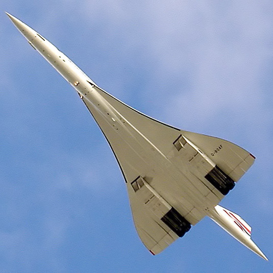
Those with even a passing knowledge of aviation history will of course be familiar with the Concorde. Jointly developed by France and Britain, the sleek aircraft has the distinction of being the only SST to achieve successful commercial operation — conducting nearly 50,000 flights between 1976 and 2003. With an average cruise speed of around Mach 2.02, it could fly up to 128 passengers from Paris to New York in just under three and a half hours.

But even before the first paying passengers climbed aboard, the Concorde put American aircraft companies such as Boeing and Lockheed into an absolute panic. It was clear that none of their SST designs could beat it to market, and there was a fear that the Concorde (and by extension, Europe) would dominate commercial supersonic flight. At least on paper, it seemed like the Concorde would quickly make subsonic long-range jetliners such as the Boeing 707 obsolete, at least for intercontinental routes. Around this time, the Soviet Union also started developing their own SST, the Tupolev Tu-144.

The perceived threat was so great that US aerospace companies started lobbying Congress to provide the funds necessary to develop an American supersonic airliner that was faster and could carry more passengers than the Concorde or Tu-144. In June of 1963, President Kennedy announced the creation of the National Supersonic Transport program during a speech at the US Air Force Academy. Four years later it was announced that Boeing’s 733-390 concept had been selected for production, and by the end of 1969, 26 airlines had put in reservations to purchase what was assumed to be the future of American air travel.

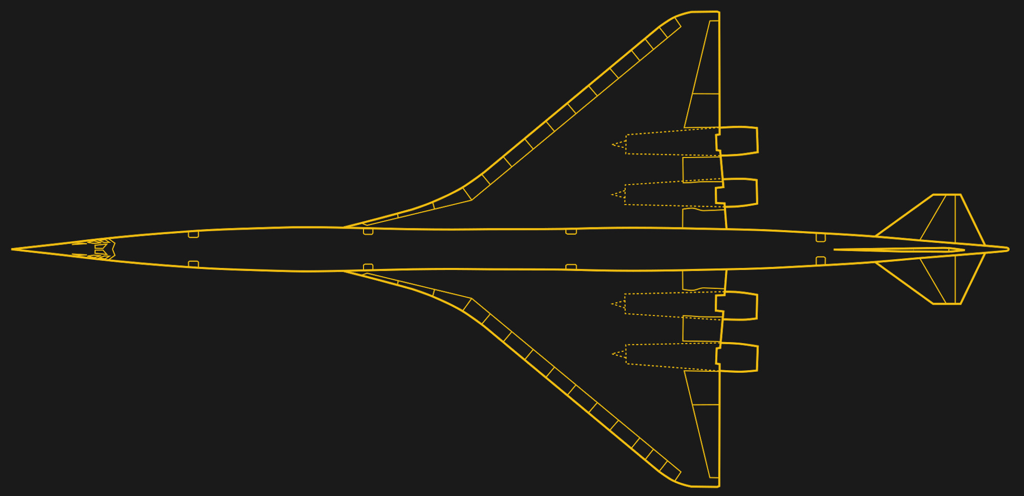
Even for a SST, the 733-390 was ambitious. It didn’t take long before Boeing started scaling back the design, first deleting the complex swing-wing mechanism for a fixed delta wing, before ultimately shrinking the entire aircraft. Even so, the redesigned aircraft (now known as the Model 2707-300) was expected to carry nearly twice as many passengers as the Concorde and travel at speeds up to Mach 3.

A Change in the Wind

But by the dawn of the 1970s it was clear that the Concorde, and the SST concept in general, wasn’t shaping up the way many in the industry expected. Even though it had yet to make its first commercial flight, demand for the Concorde among airlines was already slipping. It was initially predicted that the Concorde fleet would number as high as 350 by the 1980s, but by the time the aircraft was ready to start flying passengers, there were only 76 orders on the books.

Part of the problem was the immense cost overruns of the Concorde program, which lead to a higher sticker price on the aircraft than the airlines had initially expected. But there was also a growing concern over the viability of SSTs. A newer generation of airliners including the Boeing 747 could carry more passengers than ever, and were more fuel efficient than their predecessors. Most importantly, the public had become concerned with the idea of regular supersonic flights over their homes and communities, and imagined a future where thunderous sonic booms would crack overhead multiple times a day.

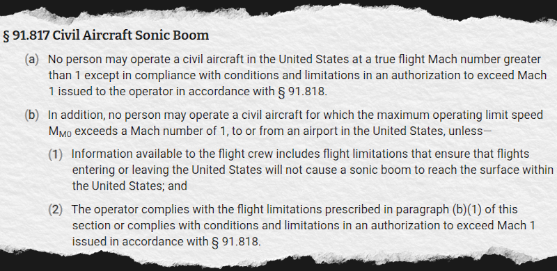
Although President Nixon supported the program, the Senate rejected any further government funding for an American SST in March of 1971. The final blow to America’s supersonic aspirations came in 1973, when the Federal Aviation Administration (FAA) enacted 14 CFR 91.817 “Civil Aircraft Sonic Boom” — prohibiting civilian flight beyond Mach 1 over the United States without prior authorization.

In the end, the SST revolution never happened. Just twenty Concorde aircraft were built, with Air France and British Airways being the only airlines that actually went through with their orders. Rather than taking over as the standard, supersonic air travel turned out to be a luxury that only a relatively few could afford.

The Silent Revolution

Since then, there have been sporadic attempts to develop a new class of civilian supersonic aircraft. But the most promising developments have only occurred in the last few years, as improved technology and advanced computer modeling has made it possible to create “low boom” supersonic aircraft. Such craft aren’t completely silent — rather than creating a single loud boom that can cause damage on the ground, they produce a series of much quieter thumps as they fly.

The Lockheed Martin X-59, developed in partnership with NASA, was designed to help explore this technology. Commercial companies such as Boom Supersonic are also developing their own takes on this concept, with eyes on eventually scaling the design up for passenger flights in the future.

In light of these developments, on June 6th President Trump signed an Executive Order titled Leading the World in Supersonic Flight which directs the FAA to repeal 14 CFR 91.817 within 180 days. In its place, the FAA is to develop a noise-based certification standard which will “define acceptable noise thresholds for takeoff, landing, and en-route supersonic operation based on operational testing and research, development, testing, and evaluation (RDT&E) data” rather than simply imposing a specific “speed limit” in the sky.

This is important, as the design of the individual aircraft as well as the environmental variables involved in the “Mach Cutoff” effect mean that there’s really no set speed at which supersonic flight becomes too loud for observers on the ground. The data the FAA will collect from these new breed of aircraft will be key in establishing reasonable noise standards which can protect the public interest without unnecessarily hindering the development of civilian supersonic aircraft.

One of the earliest commercially-successful camera technologies was the rangefinder — a rather mechanically-complex system that allows a photographer to focus by triangulating a subject, often in a dedicated focusing window, and and frame the shot with another window, all without ever actually looking through the lens. Rangefinder photographers will give you any number of reasons why their camera is just better than the others — it’s faster to use, the focusing is more accurate, the camera is lighter — but in today’s era of lightweight mirrorless digitals, all of these arguments sound like vinyl aficionados saying “The sound is just more round, man. Digital recordings are all square.” (This is being written by somebody who shoots with a rangefinder and listens to vinyl).

While there are loads of analog rangefinders floating around eBay, the trouble nowadays is that digital rangefinders are rare, and all but impossible to find for a reasonable price. Rather than complaining on Reddit after getting fed up with the lack of affordable options, [Mr.50mm] decided to do something about it, and build his own digital rangefinder for less than $250.

Part of the problem is that, aside from a few exceptions, the only digital rangefinders have been manufactured by Leica, a German company often touted as the Holy Grail of photography. Whether you agree with the hype or consider them overrated toys, they’re sure expensive. Even in the used market, you’d be hard-pressed to find an older model for less than $2,000, and the newest models can be upwards of $10,000.

Rather than start from scratch, he fused two low-cost and commonly-available cameras into one with some careful surgery and 3D printing. The digital bits came from a Panasonic GF3, a 12 MP camera that can be had for around $120, and the rangefinder system from an old Soviet camera called the Fed 5, which you can get for less than $50 if you’re lucky. The Fed 5 also conveniently worked with Leica Thread Mount (LTM) lenses, a precursor to the modern bayonet-mount lenses, so [Mr.50mm] lifted the lens mounting hardware from it as well.

Even LTM lenses are relatively cheap, as they’re not compatible with modern Leicas. Anyone who’s dabbled in building or repairing cameras will tell you that there’s loads of precision involved. If the image sensor, or film plane, offset is off by the slightest bit, you’ll never achieve a sharp focus — and that’s just one of many aspects that need to be just right. [Mr.50mm]’s attention to detail really paid off, as the sample images (which you can see in the video below) look fantastic.

With photography becoming a more expensive hobby every day, it’s great to see some efforts to build accessible and open-source cameras, and this project joins the ranks of the Pieca and this Super 8 retrofit. Maybe we’ll even see Leica-signed encrypted metadata in a future version, as it’s so easy to spoof.

It hasn’t been that long since humans figured out how to create power grids that integrated multiple generators and consumers. Ever since AC won the battle of the currents, grid operators have had to deal with the issues that come with using AC instead of the far less complex DC. Instead of simply targeting a constant voltage, generators have to synchronize with the frequency of the alternating current as it cycles between positive and negative current many times per second.

Complicating matters further, the transmission lines between generators and consumers, along with any kind of transmission equipment on the lines, add their own inductive, capacitive, and resistive properties to the system before the effects of consumers are even tallied up. The result of this are phase shifts between voltage and current that have to be managed by controlling the reactive power, lest frequency oscillations and voltage swings result in a complete grid blackout.

Flowing Backwards

We tend to think of the power in our homes as something that comes out of the outlet before going into the device that’s being powered. While for DC applications this is essentially true – aside from fights over which way DC current flows – for AC applications the answer is pretty much a “It’s complicated”. After all, the primary reason why we use AC transmission is because transformers make transforming between AC voltages easy, not because an AC grid is easier to manage.

What exactly happens between an AC generator and an AC load depends on the characteristics of the load. A major part of these characteristics is covered by its power factor (PF), which describes the effect of the load on the AC phase. If the PF is 1, the load is purely resistive with no phase shift. If the PF is 0, it’s a purely reactive load and no net current flows. Most AC-powered devices have a power factor that’s somewhere between 0.5 to 0.99, meaning that they appear to be a mixed reactive and resistive load.

PF can be understood in terms of the two components that define AC power, being:

• Apparent Power (S, in volt-amperes or VA) and
• Real Power (P, in watts).

The PF is defined as the ratio of P to S (i.e. `PF = P / S). Reactive Power (Q, in var) is easily visualized as the angle theta (Θ) between P and S if we put them as respectively the leg and hypotenuse of a right triangle. Here Θ is the phase shift by which the current waveform lags the voltage. We can observe that as the phase shift increases, the apparent power increases along with reactive power. Rather than being consumed by the load, reactive power flows back to the generator, which hints at why it’s such a problematic phenomenon for grid-management.

From the above we can deduce that the PF is 1.0 if S and P are the same magnitude. Although P = I × V gets us the real power in watts, it is the apparent power that is being supplied by the generators on the grid, meaning that reactive power is effectively ‘wasted’ power. How concerning this is to you as a consumer mostly depends on whether you are being billed for watts or VAs consumed, but from a grid perspective this is the motivation behind power factor correction (PFC).

This is where capacitors are useful, as they can correct the low PF on inductive loads like electric motors, and vice versa with inductance on capacitive loads. As a rule of thumb, capacitors create reactive power, while inductors consume reactive power, meaning that for PFC the right capacitance or inductance has to be added to get the PF as close to 1.0 as possible. Since an inductor absorbs the excess (reactive) power and a capacitor supplies reactive power, if both are balanced 1:1, the PF would be 1.0.

In the case of modern switching-mode power supplies, automatic power factor correction (APFC) is applied, which switch in capacitance as needed by the current load. This is, in miniature, pretty much what the full-scale grid does throughout the network.

Traditional Grids

Based on this essential knowledge, local electrical networks were expanded from a few streets to entire cities. From there it was only a matter of time before transmission lines turned many into few, with soon transmission networks spanning entire continents. Even so, the basic principles remain the same, and thus the methods available to manage a power grid.

Spinning generators provide the AC power, along with either the creation or absorption of reactive power on account of being inductors with their large wound coils, depending on their excitation level. Since transformers are passive devices, they will always absorb reactive power, while both overhead and underground transmission lines start off providing reactive power, overhead lines start absorbing reactive power if overloaded.

In order to keep reactive power in the grid to a healthy minimum, capacitive and inductive loads are switched in or out at locations like transmission lines and switchyards. The inductive loads often taken the form of shunt reactors – basically single winding transformers – and shunt capacitors, along with active devices like synchronous condensers that are effectively simplified synchronous generators. In locations like substations the use of tap changers enables fine-grained voltage control to ease the load on nearby transmission lines. Meanwhile the synchronous generators at thermal plants can be kept idle and online to provide significant reactive power absorption capacity when not used to actively generate power.

Regardless of the exact technologies employed, these traditional grids are characterized by significant amounts of reactive power creation and absorption capacity. As loads join or leave the grid every time that consumer devices are turned off and on, the grid manager (transmission system operator, or TSO) adjusts the state of these control methods. This keeps the grid frequency and voltage within their respective narrowly defined windows.

Variable Generators

Over the past few years, most newly added generating capacity has come in the form of weather-dependent variable generators that use grid-following converters. These devices take the DC power from generally PV solar and wind turbine farms and convert them into AC. They use a phase-locked loop (PLL) to synchronize with the grid frequency, to match this AC frequency and the current voltage.

Unfortunately, these devices do not have the ability to absorb or generate reactive power, and instead blindly follow the current grid frequency and voltage, even if said grid was going through reactive power-induced oscillations. Thus instead of damping these oscillations and any voltage swings, these converters serve to amplify these issues. During the 2025 Iberian Peninsula blackout, this was identified as one of the primary causes by the Spanish TSO.

Ultimately AC power grids depend on solid reactive power management, which is why the European group of TSOs (ENTSO-E) already recommended in 2020 that grid-following converters should get replaced with grid-forming converters. These feature the ability absorb and generate reactive power through the addition of features like energy storage and are overall significantly more useful and robust when it comes to AC grid management.

Although AC doesn’t rule the roost any more in transmission networks, with high-voltage DC now the more economical option for long distances, the overwhelming part of today’s power grids still use AC. This means that reactive power management will remain one of the most essential parts of keeping power grids stable and people happy, until the day comes when we will all be switching back to DC grids, year after the switch to AC was finally completed back in 2007.

For some reason, people are really into tiny arcade machines that basically require you to ruin your hands and eyes in order to play on them. That said, unlike the fifty gazillion ‘retro consoles’ that you can buy everywhere, the particular mini arcade machine that [David Given] of [Poking Technology] obtained from AliExpress for a teardown and ROM dump seems to have custom games rather than the typical gaggle of NES games and fifty ROM hack variations of each.

After a bit of gameplay to demonstrate the various games on the very tiny machine with tiny controls and a tiny 1.8″, 160×128 ST7735 LC display, the device was disassembled. Inside is a fairly decent speaker, the IO board for the controls, and the mainboard with an epoxy blob-covered chip and the SPI EEPROM containing the software. Dumping this  XOR ‘encrypted’ ROM was straightforward, revealing it to be a 4 MB, W23X32-compatible EEPROM.

Further reverse-engineering showed the CPU to be a WDT65C02-compatible chip, running at 8 MHz with 2 kB of SRAM and 8 kB of fast ROM in addition to a 24 MHz link to the SPI EEPROM, which is used heavily during rendering. [David] created a basic SDK for those who feel like writing their own software for this mini arcade system. Considering the market that these mini arcade systems exist in, you’ve got to give the manufacturer credit for creating a somewhat original take, with hardware that is relatively easy to mod and reprogram.

Thanks to [Clint Jay] for the tip.

The human eye’s color perception is notoriously variable (see, for example, the famous dress), which makes it difficult to standardize colours. This is where spectrophotometers come in: they measure colours reliably and repeatably, and can match them against a library of standard colors. Unfortunately, they tend to be expensive, so when Hackaday’s own [Adam Zeloof] ran across two astonishingly cheap X-Rite/Pantone RM200 spectrophotometers on eBay, he took the chance that they might still be working.

They did work, but [Adam] found that his model was intended for testing cosmetics and only had a colour library of skin tones, whereas the base model had a full colour library. This was rather limiting, but he noticed that the only apparent difference between his model and the base model was a logo (that is, a cosmetic difference). This led him to suspect that only the firmware was holding his spectrophotometer back, so he began looking for ways to install the base unit’s firmware on his device.

He started by running X-Rite’s firmware updater. Its log files revealed that it was sending the device’s serial number to an update server, which responded with the firmware information for that device. To get around this, [Adam] tried altering the updater’s network requests to send a base unit’s serial number. This seemed promising, but he also needed a device-specific security key to actually download firmware. After much searching, he managed to find a picture of a base unit showing both the serial number and security key. After substituting these values into the requests, the updater had no problem installing the base model’s firmware.

[Adam] isn’t completely sure how accurate the altered system’s measurements are, but they seem to mostly agree with his own colour calibration swatches. It’s not absolutely certain that there are no hardware differences between the models, so there might be some unknown factor producing the few aberrant results [Adam] saw. Nevertheless, this is probably accurate enough to prove that one of his roommates was wrong about the color of a gaming console.

We’ve seen a few projects before that measure and replicate existing colors. The principle’s even used to detect counterfeit bills.

So far in the “Field Guide” series, we’ve mainly looked at critical infrastructure systems that, while often blending into the scenery, are easily observable once you know where to look. From the substations, transmission lines, and local distribution systems that make up the electrical grid to cell towers and even weigh stations, most of what we’ve covered so far are mega-scale engineering projects that are critical to modern life, each of which you can get a good look at while you’re tooling down the road in a car.

This time around, though, we’re going to switch things up a bit and discuss a less-obvious but vitally important infrastructure system: the cold chain. While you might never have heard the term, you’ve certainly seen most of the major components at one time or another, and if you’ve ever enjoyed fresh fruit in the dead of winter or microwaved a frozen burrito for dinner, you’ve taken advantage of a globe-spanning system that makes sure environmentally sensitive products can be safely stored and transported.

What’s A Cold Chain?

Simply put, the cold chain is a supply chain that’s capable of handling items that are likely to be damaged or destroyed unless they’re kept within a specific temperature range. The bulk of the cold chain is devoted to products intended for human consumption, mainly food but also pharmaceuticals and vaccines. Certain non-consumables also fall under the cold chain umbrella, including cosmetics, personal care products, and even things like cut flowers and vegetable seedlings. We’ll be mainly looking at the food cold chain for this article, though, since it uses most of the major components of a cold chain.

As the name implies, the cold chain is designed to maintain a fixed temperature over the entire life of a product. “Farm to fork” is a term often used to describe the cold chain, since the moment produce is harvested or prepared foods are manufactured, the clock starts ticking. The exact temperature required varies by food type. Many fruits and vegetables that ripen in the summer or early autumn can stand pretty high temperatures, at least for a while after harvesting, but some produce, like lettuces and fresh greens, will start wilting very quickly after harvest.

For extremely sensitive crops, the cold chain might start almost the second the crop is harvested. Highly perishable crops such as sweet corn, greens, asparagus, and peas require rapid cooling to remove field heat and to slow the biological processes that were still occurring within the plant tissues at the time of harvest. This is often accomplished right in the field with a hydrocooler, which uses showers or flumes of chilled water. Extremely perishable crops such as broccoli might even be placed directly into flaked ice in the field. Other, less-sensitive crops that can wait an hour or two will enter the cold chain only when they’re trucked a short distance to an initial processing plant.

Many foods, including different kinds of produce, fresh meat and fish, and lots of prepared meals, benefit from flash freezing. Flash freezing aims to reduce damage to the food by controlling the size and number of ice crystals that form within the cells of the plant or animal tissue. Simply putting a food item in a freezer and waiting for the heat to passively transfer out of it tends to form few but large ice crystals, which are far more damaging than the many tiny ice crystals that form when the heat is rapidly removed. Flash freezing methods include cryogenic baths using liquid nitrogen or liquid carbon dioxide, blast cooling with high-velocity jets of chilled air, fluidized bed cooling, where pressurized chilled air is directed upward through a bed of produce while it’s being agitated, and plate cooling, where chilled metal plates lightly contact flat, thin foods such as pizza or sliced fish.

Big and Cold

Once food is chilled to the proper temperature, it needs to be kept at that temperature until it can be sold. This is where cold warehousing comes in, an important part of the cold chain that provides controlled-temperature storage space that individual producers simply can’t afford to maintain. The problem for farmers is that many crops are determinate, meaning that all the fruits or vegetables are ready for harvest more or less at the same time. Outsourcing their cold warehousing to companies that specialize in that part of the cold chain allows them to concentrate on growing and harvesting their crop instead of having to maintain a huge amount of storage space, which would sit unused for the entire growing season.

Cold warehouses, or public refrigerated warehouses (PRWs) as they’re known in the trade, benefit greatly from economies of scale, and since they accept produce from hundreds or even thousands of producers, their physical footprints can be staggering. The average PRW in the United States has grown in size dramatically since the post-pandemic e-commerce boom and now covers almost 185,000 square feet, or more than 4 acres. Most PRWs have four temperature zones: deep freeze (-20°F to -10°F) for items such as ice cream and frozen vegetables; freezer (0°F to 10°F) for meats and prepared foods; refrigerated (35°F to 45°F), for fresh fruits and vegetables; and cool storage, which is basically just consistent room-temperature storage for shelf-stable food items. What’s more, each zone can have sub-zones tailored specifically for foods that prefer a specific temperature; bananas, for example, do best around 46°F, making the fridge section too cold and the cool section too warm. Sub-zones allow goods to be stored just right.

Due to the nature of their business, location is critical to PRWs. They have to be close to where the food is produced as well as handy to transportation hubs, which means you’ve probably seen one of these behemoth buildings from a highway and not even known it. The map above highlights the main agricultural regions of the United States, such as the fruit and vegetable producers in the Central Valley of California and the Willamette Valley in Oregon, meat packing plants in the Upper Midwest, the hog and chicken producers in the South, and seafood producers along both coasts. It also shows a couple of areas with no PRWs, which are areas where agriculture is limited to cereal grains, which don’t require refrigeration after harvest, and livestock, which are usually shipped for slaughter somewhere other than where they were raised.

Thanks to the complicated logistics of managing multiple shippers and receivers, most cold warehouses have a level of automation that rivals that of an Amazon distribution center. A lot of the automation is found in the high-bay freezer, a space often three or four stories tall that has rack after rack of space for storing palletized products. Automated storage and retrieval systems (AS/RS) store and fetch pallets using large X-Y gantry systems running between the racks. Algorithms determine the best storage location for pallets based on their contents, the temperature regime they require, and the predicted length of stay within the warehouse.

While AS/RS reduces the number of workers needed to run a cold warehouse, and there are some fully automated PRWs, most cold warehouses maintain a large workforce to run forklifts, pick pallets, and assemble orders for shipping. These workers face significant health and safety challenges, risking everything from slips and falls on icy patches to trench foot and chill-induced arthritis and dermatitis. Cold-stress injuries, such as hypothermia and frostbite, are possible too. Warehouses often have to limit the number of hours their employees work in the cold zones, and they have to provide thermal wear along with the standard complement of PPE.

Reefer Madness

Once an order is assembled and ready to ship from the cold warehouse, food enters perhaps the most visible — and riskiest — link in the cold chain: refrigerated trucks and shipping containers. Known as reefers, these are specialized vehicles that have the difficult task of keeping their contents at a constant temperature no matter what the outside conditions might be. A reefer might have to deliver a load of table grapes from a PRW in California to a supermarket distribution center in Massachusetts, continue to Maine to pick up a load of live lobsters, and drop that off at a PRW in Florida before running a load of oranges to Washington.

Meeting the challenge of all these conditions is the job of the refrigeration unit. Typically mounted in an aerodynamic fairing on the front of a semi-trailer unit, the refrigeration unit is essentially a heat pump on steroids. For over-the-road (OTR) reefers, as opposed to railcar reefers or shipping container reefers, the refrigeration unit is powered by a small but powerful diesel engine. Typically either three- or four-cylinder engines making 20 to 30 horsepower, these engines run the compressor that pumps the refrigerant through the condenser and evaporator, as well as the powerful fan that circulates air inside the trailer. Fuel for the engine is stored in a tank mounted under the trailer, allowing the reefer to run even when the trailer is parked with no tractor attached. The refrigeration unit is completely automatic, with a computer taking input from temperature sensors inside the trailer to make sure the interior remains at the setpoint. The computer also logs everything going on in the reefer, making the data available via a USB drive or to a central dispatcher via a telematics link.

The trailer body itself is carefully engineered, with thick insulation to minimize heat transfer to and from the outside environment while maximizing heat transfer between the produce and the air inside the trailer. For maximum cooling — or heating; if a load of bananas has to be kept at their happy place of 46°F while being trucked across eastern Wyoming in January, the refrigeration unit will probably have to run its cycle in reverse to add heat to the trailer — the air must reach the back of the unit. Reefer units use flexible ducts in the ceiling to direct the air 48 to 53 feet to the very back of the trailer, where it bounces off the rear doors and returns to the front of the trailer with the help of channels built into the floor. Shippers need to be careful when loading a reefer to obey load height limits and to correctly orient pallets so as not to block air circulation inside the trailer.

In addition to the data logging provided by the refrigeration unit, shippers will often include temperature loggers inside their shipments. Known generically to produce truckers as a “Ryan” for a popular brand, these analog strip chart recorders use a battery-powered motor to move a strip of paper past a bimetallic arm. Placed in a tamper-evident container, the recorder is placed within a pallet and records the temperature over a 10- to 40-day period. The receiver can break the seal open and see a complete temperature history of the shipment, detecting any accidental (or intentional; drivers sometimes find it hard to sleep with the reefer motor roaring right behind the sleeper cab) interruptions in the operation of the reefer.

Featured image: “Close Up of Frozen Vegetables” by Tohid Hashemkhani

If you are looking for the perfect instrument to start a biological horror show in our age of AI, you have come to the right place. Researchers at Johns Hopkins University have successfully used AI-guided robotics to perform surgical procedures. So maybe a bit less dystopian, but the possibilities are endless.

Pig parts are used as surrogate human gallbladders to demonstrate cholecystectomies. The skilled surgeon is replaced with a Da Vinci research kit, similarly used in human controlled surgeries.

Researchers used an architecture that uses live imaging and human corrections to input into a high-level language model, which feeds into the controlling low-level model. While there is the option to intervene with human input, the model is trained to and has demonstrated the ability to self-correct. This appears to work fairly well with nothing but minor errors, as shown in an age-restricted YouTube video. (NOTE: SURGICAL IMAGERY WATCH AT YOUR OWN RISK)

It’s noted that the robot performed slower than a traditional surgeon, trading time for precision. As always, when talking about anything medical, it’s not likely we will be seeing it on our own gallbladders anytime soon, but maybe within the next decade. If you want to read more on the specific advancements, check out the paper here.

Medical hacking isn’t always the most appealing for anyone with a weak stomach. For those of us with iron guts make sure to check out this precision tendon tester!

There are a lot of benefits to writing for Hackaday, but hands down one of the best is getting paid to fall down fascinating rabbit holes. These often — but not always — delightful journeys generally start with chance comments by readers, conversations with fellow writers, or just the random largesse of The Algorithm. Once steered in the right direction, a few mouse clicks are all it takes for the properly prepared mind to lose a few hours chasing down an interesting tale.

I’d like to say that’s exactly how this article came to be, but to be honest, I have no idea where I first heard about the prison camp lathe. I only know that I had a link to a PDF of an article written in 1949, and that was enough to get me going. It was probably a thread I shouldn’t have tugged on, but I’m glad I did because it unraveled into a story not only of mechanical engineering chops winning the day under difficult circumstances, but also of how ingenuity and determination can come together to make the unbearable a little less trying, and how social engineering is an important a skill if you want to survive the unsurvivable.

Finding Reggie

For as interesting a story as this is, source material is hard to come by. Searches for “prison camp lathe” all seem to point back to a single document written by one “R. Bradley, A.M.I.C.E” in 1949, describing the building of the lathe. The story, which has been published multiple times in various forms over the ensuing eight decades, is a fascinating read that’s naturally heavy on engineering details, given the subject matter and target audience. But one suspects there’s a lot more to the story, especially from the few tantalizing details of the exploits surrounding the tool’s creation that R. Bradley floats.

Tracking down more information about Bradley’s wartime experiences proved difficult, but not impossible. Thankfully, the United Kingdom’s National Archives Department has an immense trove of information from World War II, including a catalog of the index cards used by the Japanese Empire to keep track of captured Allied personnel. The cards are little more than “name, rank, and serial number” affairs, but that was enough to track down a prisoner named Reginald Bradley:

Now, it’s true that Reginald Bradley is an extremely British name, and probably common enough that this wasn’t the only Reggie Bradley serving in the Far East theater in World War II. And while the date of capture, 15 February 1942, agrees with the date listed in the lathe article, it also happens to be the date of the Fall of Singapore, the end of a seven-day battle between Allied (mainly British) forces and the Japanese Imperial Army and Navy that resulted in the loss of the island city-state. About 80,000 Allied troops were captured that day, increasing the odds of confusing this Reginald Bradley with the R. Bradley who wrote the article.

The clincher, though, is Reginald Bradley’s listed occupation on the prisoner card: “Chartered Civil Engineer.” Even better is the information captured in the remarks field, which shows that this prisoner is an Associate Member of the Institution of Civil Engineers, which agrees with the “A.C.I.M.E” abbreviation in the article’s byline. Add to that the fact that the rank of Captain in the Royal Artillery listed on the card agrees with the author’s description of himself, and it seems we have our man. (Note: it’s easy to fall into the genealogical rabbit hole at this point, especially with an address and mother’s name to work with. Trust me, though; that way lies madness. It’s enough that the index card pictured above cost me £25 to retrieve from one of the National Archive’s “trusted partner” sites.)

The Royal Society of Social Engineers

The first big question about Captain Bradley is how he managed to survive his term as a prisoner of the Japanese Empire, which, as a non-signatory to the various international conventions and agreements on the treatment of prisoners of war, was famed for its poor treatment of POWs. Especially egregious was the treatment of prisoners assigned to build the Burma Death Railway, an infrastructure project that claimed 45 lives for every mile of track built. Given that his intake card clearly states his civil engineering credentials with a specialty in highways and bridges, one would think he was an obvious choice to be sent out into the jungle.

Rather than suffering that fate, Captain Bradley was sent to the infamous prison camp that had been established in Singapore’s Changi Prison complex. While not pleasant, it was infinitely preferable to the trials of the jungle, but how Bradley avoided that fate is unclear, as he doesn’t mention the topic at all in his article. He does, however, relate a couple of anecdotes that suggest that bridges and highways weren’t his only engineering specialty. Captain Bradley clearly had some social engineering chops too, which seem to have served him in good stead during his internment.

Within the first year of his term, he and his fellow officers had stolen so many tools from their Japanese captors that it was beginning to be a problem to safely stash their booty. They solved the problem by chatting up a Japanese guard under the ruse of wanting to learn a little Japanese. After having the guard demonstrate some simple pictograms like “dog” and “tree,” they made the leap to requesting the symbol for “workshop.” Miraculously, the guard fell for it and showed them the proper strokes, which they copied to a board and hung outside the officer’s hut between guard changes. The new guard assumed the switch from hut to shop was legitimate, and the prisoners could finally lay out all their tools openly and acquire more.

Another bit of social engineering that Captain Bradley managed, and probably what spared him from railway work, was his reputation as a learned man with a wide variety of interests. This captured the attention of a Japanese general, who engaged the captain in long discussions on astronomy. Captain Bradley appears to have cultivated this relationship carefully, enough so that he felt free to gripe to the general about the poor state of the now officially sanctioned workshop, which had been moved to the camp’s hospital block. A care package of fresh tools and supplies, including drill bits, hacksaw blades, and a supply of aluminum rivets, which would prove invaluable, soon arrived. These joined their pilfered tool collection along with a small set of machines that were in the original hospital shop, which included a hand-operated bench drill, a forge, some vises, and crucially, a small lathe. This would prove vital in the efforts to come, but meanwhile, the shop’s twelve prisoner-machinists were put to work making things for the hospital, mainly surgical instruments and, sadly, prosthetic limbs.

The Purdon Joint

In his article, Captain Bradley devotes curiously little space to descriptions of these prosthetics, especially since he suggests that his “link-motion” design was innovative enough that prisoners who had lost legs to infection, a common outcome even for small wounds given the poor nutrition and even poorer sanitation in the camps, were able to walk well enough that a surgeon in the camp, a British colonel, noted that “It is impossible to tell that the walker is minus a natural leg.” The lack of detail on the knee’s design might also be due to modesty, since other descriptions of these prostheses credit the design of the knee joint to Warrant Officer Arthur Henry Mason Purdon, who was interned at Changi during this period.

A number of examples of the prosthetic legs manufactured at “The Artificial Limb Factory,” as the shop was now dubbed, still exist in museum collections today. The consensus design seems to accommodate below-the-knee amputees with a leather and canvas strap for the thigh, a hinge to transfer most of the load from the lower leg to the thigh around the potentially compromised knee, a calf with a stump socket sculpted from aluminum, and a multi-piece foot carved from wood. The aluminum was often salvaged from downed aircraft, hammered into shape and riveted together. When the gifted supply of aluminum rivets was depleted, Bradley says that new ones were made on the lathe using copper harvested from heavy electrical cables in the camp.

It Takes a Lathe to Make a Lathe

While the Limb Factory was by now a going concern that produced items necessary to prisoners and captors alike, life in a prison camp is rarely fair, and the threat of the entire shop being dismantled at any moment weighed heavily on Captain Bradley and his colleagues. That’s what spurred the creation of the lathe detailed in Bradley’s paper — a lathe that the Japanese wouldn’t know about, and that was small enough to hide quickly, or even stuff into a pack and take on a forced march.

The paper goes into great detail on the construction of the lathe, which started with the procurement of a scrap of 3″ by 3″ steel bar. Cold chisels and drills were used to shape the metal before surfacing it on one of the other lathes using a fly cutter. Slides were similarly chipped from 1/2″ thick plate, and when a suitable piece of stock for the headstock couldn’t be found, one was cast from scrap aluminum using a sand mold in a flask made from sheet steel harvested from a barracks locker.

Between his other shop duties and the rigors of prison life, Captain Bradley continued his surreptitious work on the lathe, and despite interruptions from camp relocations, was able to complete it in about 600 hours spread over six months. He developed ingenious ways to power the lathe using old dynamos and truck batteries. The lathe was used for general maintenance work in the shop, such as making taps and dies to replace worn and broken ones from the original gift of tools bequeathed by the Japanese general.

With the end of the war approaching, the lathe was put to use making the mechanical parts needed for prison camp radios, some of which were ingeniously hidden in wooden beams of the barracks or even within the leg of a small table. The prisoners used these sets to listen for escape and evasion orders from Allied command, or to just get any news of when their imprisonment might be over.

That day would come soon after the atomic bombing of Hiroshima and Nagasaki and Japan’s subsequent surrender in August 1945. The Changi prison camp was liberated about two weeks later, with the survivors returning first to military and later to civilian life. Warrant Officer Purdon, who was already in his 40s when he enlisted, was awarded a Distinguished Combat Medal for his courage during the Battle of Singapore. As for Captain Bradley, his trail goes cold after the war, and there don’t seem to be any publicly available pictures of him. He was decorated by King George VI after the war, though, “for gallant and distinguished service while a prisoner of war,” as were most other POWs. The award was well-earned, of course, but an understatement in the extreme for someone who did so much to lighten the load of his comrades in arms.

Featured image: “Warrant Officer Arthur Henry Mason Purdon, Changi Prison Camp, Singapore. c. 1945“, Australian War Memorial.

Normally you can’t read out the One Time Programming (OTP) memory in Microchip’s PIC MCUs that have code protection enabled, but an exploit has been found that gets around the copy protection in a range of PIC12, PIC14 and PIC16 MCUs.

This exploit is called PIC Burnout, and was developed by [Prehistoricman], with the cautious note that although this process is non-invasive, it does damage the memory contents. This means that you likely will only get one shot at dumping the OTP data before the memory is ‘burned out’.

The copy protection normally returns scrambled OTP data, with an example of PIC Burnout provided for the PIC16LC63A. After entering programming mode by setting the ICSP CLK pin high, excessively high programming voltage and duration is used repeatedly while checking that an area that normally reads as zero now reads back proper data. After this the OTP should be read out repeatedly to ensure that the scrambling has been circumvented.

The trick appears to be that while there’s over-voltage and similar protections on much of the Flash, this approach can still be used to affect the entire flash bit column. Suffice it to say that this method isn’t very kind to the Flash memory cells and can take hours to get a good dump. Even after this you need to know the exact scrambling method used, which is fortunately often documented by Microchip datasheets.

Thanks to [DjBiohazard] for the tip.

AF114 germanium transistors and related ones like the AF115 through AF117 were quite popular during the 1960s, but they quickly developed a reputation for failure. This is due to what should have made them more reliable, namely the can shielding the germanium transistor inside that is connected with a fourth ‘screen’ pin. This failure mode is demonstrated in a video by [Anthony Francis-Jones] in which he tests a number of new-old-stock AF-series transistors only for them all to test faulty and show clear whisker growth on the can’s exterior.

Naturally, the next step was to cut one of these defective transistors open to see whether the whiskers could be caught in the act. For this a pipe cutter was used on the fairly beefy can, which turned out to rather effective and gave great access to the inside of these 1960s-era components. The insides of the cans were as expected bristling with whiskers.

The AF11x family of transistors are high-frequency PNP transistors that saw frequent use in everything from consumer radios to just about anything else that did RF or audio. It’s worth noting that the material of the can is likely to be zinc and not tin, so these would be zinc whiskers. Many metals like to grow such whiskers, including lead, so the end effect is often a thin conductive strand bridging things that shouldn’t be. Apparently the can itself wasn’t the only source of these whiskers, which adds to the fun.

In the rest of the video [Anthony] shows off the fascinating construction of these germanium transistors, as well as potential repairs to remove the whisker-induced shorts through melting them. This is done by jolting them with a fairly high current from a capacitor. The good news is that this made the component tester see the AF114 as a transistor again, except as a rather confused NPN one. Clearly this isn’t an easy fix, and it would be temporary at best anyway, as the whiskers will never stop growing.

Who knows what you’ll find in a second-hand shop? [Zeal] found some old keyboards made to fit early Alcatel phones from the year 2000 or so. They looked good but, of course, had no documentation. He’s made two videos about his adventure, and you can see them below.

The connector was a cellphone-style phone jack that must carry power and some sort of serial data. Inside, there wasn’t much other than a major chip and a membrane keyboard. There were a few small support chips and components, too.

This is a natural job for a logic analyzer. Sure enough, pressing a key showed some output on the logic analyzer. The device only outputs data, and so, in part 2, [Zeal] adds it to his single-board Z-80 computer.

It makes a cute package, but it did take some level shifting to get the 5V logic to play nice with the lower-voltage keyboard. He used a processor to provide protocol translation, although it looks like you could have easily handled the whole thing in the host computer software if you had wanted to do so.

Truthfully, there isn’t much chance you are going to find this exact keyboard. However, the process of opening a strange device and reverse engineering what it is all about is classic.

Don’t have a logic analyzer? A scope might have been usable for this, but you can also build one for very little these days. Using a PS/2 keyboard isn’t really easier, by the way, it is just well-documented.

[Hunter Irving] is a talented hacker with a wicked sense of humor, and he has written in to let us know about his latest project which is to make a GameCube keyboard controller work with Animal Crossing.

This project began simply enough but got very complicated in short order. Initially the goal was to get the GameCube keyboard controller integrated with the game Animal Crossing. The GameCube keyboard controller is a genuine part manufactured and sold by Nintendo but the game Animal Crossing isn’t compatible with this controller. Rather, Animal Crossing has an on-screen keyboard which players can use with a standard controller. [Hunter] found this frustrating to use so he created an adapter which would intercept the keyboard controller protocol and replace it with equivalent “keypresses” from an emulated standard controller.

In this project [Hunter] intercepts the controller protocol and the keyboard protocol with a Raspberry Pi Pico and then forwards them along to an attached GameCube by emulating a standard controller from the Pico. Having got that to work [Hunter] then went on to add a bunch of extra features.

First he designed and 3D-printed a new set of keycaps to match the symbols available in the in-game character set and added support for those. Then he made a keyboard mode for entering musical tunes in the game. Then he integrated a database of cheat codes to unlock most special items available in the game. Then he made it possible to import images (in low-resolution, 32×32 pixels) into the game. Then he made it possible to play (low-resolution) videos in the game. And finally he implemented a game of Snake, in-game! Very cool.

If you already own a GameCube and keyboard controller (or if you wanted to get them) this project would be good fun and doesn’t demand too much extra hardware. Just a Raspberry Pi Pico, two GameCube controller cables, two resistors, and a Schottky diode. And if you’re interested in Animal Crossing you might enjoy getting it to boot Linux!

Thanks very much to [Hunter] for writing in to let us know about this project. Have your own project? Let us know on the tipsline!

A lot of people complain that driving across the United States is boring. Having done the coast-to-coast trip seven times now, I can’t agree. Sure, the stretches through the Corn Belt get a little monotonous, but for someone like me who wants to know how everything works, even endless agriculture is fascinating; I love me some center-pivot irrigation.

One thing that has always attracted my attention while on these long road trips is the weigh stations that pop up along the way, particularly when you transition from one state to another. Maybe it’s just getting a chance to look at something other than wheat, but weigh stations are interesting in their own right because of everything that’s going on in these massive roadside plazas. Gone are the days of a simple pull-off with a mechanical scale that was closed far more often than it was open. Today’s weigh stations are critical infrastructure installations that are bristling with sensors to provide a multi-modal insight into the state of the trucks — and drivers — plying our increasingly crowded highways.

All About the Axles

Before diving into the nuts and bolts of weigh stations, it might be helpful to discuss the rationale behind infrastructure whose main function, at least to the casual observer, seems to be making the truck driver’s job even more challenging, not to mention less profitable. We’ve all probably sped by long lines of semi trucks queued up for the scales alongside a highway, pitying the poor drivers and wondering if the whole endeavor is worth the diesel being wasted.

The answer to that question boils down to one word: axles. In the United States, the maximum legal gross vehicle weight (GVW) for a fully loaded semi truck is typically 40 tons, although permits are issued for overweight vehicles. The typical “18-wheeler” will distribute that load over five axles, which means each axle transmits 16,000 pounds of force into the pavement, assuming an even distribution of weight across the length of the vehicle. Studies conducted in the early 1960s revealed that heavier trucks caused more damage to roadways than lighter passenger vehicles, and that the increase in damage is proportional to the fourth power of axle weight. So, keeping a close eye on truck weights is critical to protecting the highways.

Just how much damage trucks can cause to pavement is pretty alarming. Each axle of a truck creates a compression wave as it rolls along the pavement, as much as a few millimeters deep, depending on road construction and loads. The relentless cycle of compression and expansion results in pavement fatigue and cracks, which let water into the interior of the roadway. In cold weather, freeze-thaw cycles exert tremendous forces on the pavement that can tear it apart in short order. The greater the load on the truck, the more stress it puts on the roadway and the faster it wears out.

The other, perhaps more obvious reason to monitor axles passing over a highway is that they’re critical to truck safety. A truck’s axles have to support huge loads in a dynamic environment, and every component mounted to each axle, including springs, brakes, and wheels, is subject to huge forces that can lead to wear and catastrophic failure. Complete failure of an axle isn’t uncommon, and a driver can be completely unaware that a wheel has detached from a trailer and become an unguided missile bouncing down the highway. Regular inspections of the running gear on trucks and trailers are critical to avoiding these potentially catastrophic occurrences.

Ways to Weigh

The first thing you’ll likely notice when driving past one of the approximately 700 official weigh stations lining the US Interstate highway system is how much space they take up. In contrast to the relatively modest weigh stations of the past, modern weigh stations take up a lot of real estate. Most weigh stations are optimized to get the greatest number of trucks processed as quickly as possible, which means constructing multiple lanes of approach to the scale house, along with lanes that can be used by exempt vehicles to bypass inspection, and turnout lanes and parking areas for closer inspection of select vehicles.

In addition to the physical footprint of the weigh station proper, supporting infrastructure can often be seen miles in advance. Fixed signs are usually the first indication that you’re getting near a weigh station, along with electronic signboards that can be changed remotely to indicate if the weigh station is open or closed. Signs give drivers time to figure out if they need to stop at the weigh station, and to begin the process of getting into the proper lane to negotiate the exit. Most weigh stations also have a net of sensors and cameras mounted to poles and overhead structures well before the weigh station exit. These are monitored by officers in the station to spot any trucks that are trying to avoid inspections.

Most weigh stations in the US are located off the right side of the highway, as left-hand exit ramps are generally more dangerous than right exits. Still, a single weigh station located in the median of the highway can serve traffic from both directions, so the extra risk of accidents from exiting the highway to the left is often outweighed by the savings of not having to build two separate facilities. Either way, the main feature of a weigh station is the scale house, a building with large windows that offer a commanding view of the entire plaza as well as an up-close look at the trucks passing over the scales embedded in the pavement directly adjacent to the structure.

Scales at a weigh station are generally of two types: static scales, and weigh-in-motion (WIM) systems. A static scale is a large platform, called a weighbridge, set into a pit in the inspection lane, with the surface flush with the roadway. The platform floats within the pit, supported by a set of cantilevers that transmit the force exerted by the truck to electronic load cells. The signal from the load cells is cleaned up by signal conditioners before going to analog-to-digital converters and being summed and dampened by a scale controller in the scale house.

The weighbridge on a static scale is usually long enough to accommodate an entire semi tractor and trailer, which accurately weighs the entire vehicle in one measurement. The disadvantage is that the entire truck has to come to a complete stop on the weighbridge to take a measurement. Add in the time it takes for the induced motion of the weighbridge to settle, along with the time needed for the driver to make a slow approach to the scale, and each measurement can add up to significant delays for truckers.

To avoid these issues, weigh-in-motion systems are often used. WIM systems use much the same equipment as the weighbridge on a static scale, although they tend to use piezoelectric sensors rather than traditional strain-gauge load cells, and usually have a platform that’s only big enough to have one axle bear on it at a time. A truck using a WIM scale remains in motion while the force exerted by each axle is measured, allowing the controller to come up with a final GVW as well as weights for each axle. While some WIM systems can measure the weight of a vehicle at highway speed, most weigh stations require trucks to keep their speed pretty slow, under five miles per hour. This is obviously for everyone’s safety, and even though the somewhat stately procession of trucks through a WIM can still plug traffic up, keeping trucks from having to come to a complete stop and set their brakes greatly increases weigh station throughput.

Another advantage of WIM systems is that the spacing between axles can be measured. The speed of the truck through the scale can be measured, usually using a pair of inductive loops embedded in the roadway around the WIM sensors. Knowing the vehicle’s speed through the scale allows the scale controller to calculate the distance between axles. Some states strictly regulate the distance between a trailer’s kingpin, which is where it attaches to the tractor, and the trailer’s first axle. Trailers that are not in compliance can be flagged and directed to a parking area to await a service truck to come by to adjust the spacing of the trailer bogie.

Keep It Moving, Buddy

Despite the increased throughput of WIM scales, there are often too many trucks trying to use a weigh station at peak times. To reduce congestion further, some states participate in automatic bypass systems. These systems, generically known as PrePass for the specific brand with the greatest market penetration, use in-cab transponders that are interrogated by transmitters mounted over the roadway well in advance of the weigh station. The transponder code is sent to PrePass for authentication, and if the truck ID comes back to a company that has gone through the PrePass certification process, a signal is sent to the transponder telling the driver to bypass the weigh station. The transponder lights a green LED in this case, which stays lit for about 15 minutes, just in case the driver gets stopped by an overzealous trooper who mistakes the truck for a scofflaw.

PrePass transponders are just one aspect of an entire suite of automatic vehicle identification (AVI) systems used in the typical modern weigh station. Most weigh stations are positively bristling with cameras, some of which are dedicated to automatic license plate recognition. These are integrated into the scale controller system and serve to associate WIM data with a specific truck, so violations can be flagged. They also help with the enforcement of traffic laws, as well as locating human traffickers, an increasingly common problem. Weigh stations also often have laser scanners mounted on bridges over the approach lanes to detect unpermitted oversized loads. Image analysis systems are also used to verify the presence and proper operation of required equipment, such a mirrors, lights, and mudflaps. Some weigh stations also have systems that can interrogate the electronic logging device inside the cab to verify that the driver isn’t in violation of hours of service laws, which dictate how long a driver can be on the road before taking breaks.

Sensors Galore

Another set of sensors often found in the outer reaches of the weigh station plaza is related to the mechanical status of the truck. Infrared cameras are often used to scan for excessive heat being emitted by an axle, often a sign of worn or damaged brakes. The status of a truck’s tires can also be monitored thanks to Tire Anomaly and Classification Systems (TACS), which use in-road sensors that can analyze the contact patch of each tire while the vehicle is in motion. TACS can detect flat tires, over- and under-inflated tires, tires that are completely missing from an axle, or even mismatched tires. Any of these anomalies can cause a tire to quickly wear out and potentially self-destruct at highway speeds, resulting in catastrophic damage to surrounding traffic.

Trucks with problems are diverted by overhead signboards and direction arrows to inspection lanes. There, trained truck inspectors will closely examine the flagged problem and verify the violation. If the problem is relatively minor, like a tire inflation problem, the driver might be able to fix the issue and get back on the road quickly. Trucks that can’t be made safe immediately might have to wait for mobile service units to come fix the problem, or possibly even be taken off the road completely. Only after the vehicle is rendered road-worthy again can you keep on trucking.

Featured image: “WeighStationSign” by [Wasted Time R]

It’s an inconvenient fact that most of Earth’s largesse of useful minerals is locked up in, under, and around a lot of rock. Our little world condensed out of the remnants of stars whose death throes cooked up almost every element in the periodic table, and in the intervening billions of years, those elements have sorted themselves out into deposits that range from the easily accessed, lying-about-on-the-ground types to those buried deep in the crust, or worse yet, those that are distributed so sparsely within a mineral matrix that it takes harvesting megatonnes of material to find just a few kilos of the stuff.

Whatever the substance of our desires, and no matter how it is associated with the rocks and minerals below our feet, almost every mining and refining effort starts with wresting vast quantities of rock from the Earth’s crust. And the easiest, cheapest, and fastest way to do that most often involves blasting. In a very real way, explosives make the world work, for without them, the minerals we need to do almost anything would be prohibitively expensive to produce, if it were possible at all. And understanding the chemistry, physics, and engineering behind blasting operations is key to understanding almost everything about Mining and Refining.

First, We Drill

For almost all of the time that we’ve been mining minerals, making big rocks into smaller rocks has been the work of strong backs and arms supplemented by the mechanical advantage of tools like picks, pry bars, and shovels. The historical record shows that early miners tried to reduce this effort with clever applications of low-energy physics, such as jamming wooden plugs into holes in the rocks and soaking them with liquid to swell the wood and exert enough force to fracture the rock, or by heating the rock with bonfires and then flooding with cold water to create thermal stress fractures. These methods, while effective, only traded effort for time, and only worked for certain types of rock.

Mining productivity got a much-needed boost in 1627 with the first recorded use of gunpowder for blasting at a gold mine in what is now Slovakia. Boreholes were stuffed with powder that was ignited by a fuse made from a powder-filled reed. The result was a pile of rubble that would have taken weeks to produce by hand, and while the speed with which the explosion achieved that result was probably much welcomed by the miners, in reality, it only shifted their efforts to drilling the boreholes, which generally took a five-man crew using sledgehammers and striker bars to pound deep holes into the rock. Replacing that manual effort with mechanical drilling was the next big advance, but it would have to wait until the Industrial Revolution harnessed the power of steam to run drills capable of boring deep holes in rock quickly and with much smaller crews.

The basic principles of rock drilling developed in the 19th century, such as rapidly spinning a hardened steel bit while exerting tremendous down-pressure and high-impulse percussion, remain applicable today, although with advancements like synthetic diamond tooling and better methods of power transmission. Modern drills for open-cast mining fall into two broad categories: overburden drills, which typically drill straight down or at a slight angle to vertical and can drill large-diameter holes over 100 meters deep, and quarry drills, which are smaller and more maneuverable rigs that can drill at any angle, even horizontally. Most drill rigs are track-driven for greater mobility over rubble-strewn surfaces, and are equipped with soundproofed, air-conditioned cabs with safety cages to protect the operator. Automation is a big part of modern rigs, with automatic leveling systems, tool changers that can select the proper bit for the rock type, and fully automated drill chain handling, including addition of drill rod to push the bit deeper into the rock. Many drill rigs even have semi-autonomous operation, where a single operator can control a fleet of rigs from a single remote control console.

Proper Prior Planning

While the use of explosives seems brutally chaotic and indiscriminate, it’s really the exact opposite. Each of the so-called “shots” in a blasting operation is a carefully controlled, highly engineered event designed to move material in a specific direction with the desired degree of fracturing, all while ensuring the safety of the miners and the facility.

To accomplish this, a blasting plan is put together by a mining engineer. The blasting plan takes into account the mechanical characteristics of the rock, the location and direction of any pre-existing fractures or faults, and proximity to any structures or hazards. Engineers also need to account for the equipment used for mucking, which is the process of removing blasted material for further processing. For instance, a wheeled loader operating on the same level, or bench, that the blasting took place on needs a different size and shape of rubble pile than an excavator or dragline operating from the bench above. The capabilities of the rock crushing machinery that’s going to be used to process the rubble also have to be accounted for in the blasting plan.

Most blasting plans define a matrix of drill holes with very specific spacing, generally with long rows and short columns. The drill plan specifies the diameter of each hole along with its depth, which usually goes a little beyond the distance to the next bench down. The mining engineer also specifies a stem height for the hole, which leaves room on top of the explosives to backfill the hole with drill tailings or gravel.

Prills and Oil

Once the drill holes are complete and inspected, charging the holes with explosives can begin. The type of blasting agents to be used is determined by the blasting plan, but in most cases, the agent of choice is ANFO, or ammonium nitrate and fuel oil. The ammonium nitrate, which contains 60% oxygen by weight, serves as an oxidizer for the combustion of the long-chain alkanes in the fuel oil. The ideal mix is 94% ammonium nitrate to 6% fuel oil.

How the ANFO is added to the hole depends on conditions. For holes where groundwater is not a problem, ammonium nitrate in the form of small porous beads or prills, is poured down the hole and lightly tamped to remove any voids or air spaces before the correct amount of fuel oil is added. For wet conditions, an ammonium nitrate emulsion will be used instead. This is just a solution of ammonium nitrate in water with emulsifiers added to allow the fuel oil to mix with the oxidizer.

ANFO is classified as a tertiary explosive, meaning it is insensitive to shock and requires a booster to detonate. The booster charge is generally a secondary explosive such as PETN, or pentaerythritol tetranitrate, a powerful explosive that’s chemically similar to nitroglycerine but is much more stable. PETN comes in a number of forms, with cardboard cylinders like oversized fireworks or a PETN-laced gel stuffed into a plastic tube that looks like a sausage being the most common.

Being a secondary explosive, the booster charge needs a fairly strong shock to detonate. This shock is provided by a blasting cap or detonator, which is a small, multi-stage pyrotechnic device. These are generally in the form of a small brass or copper tube filled with a layer of primary explosive such as lead azide or fulminate of mercury, along with a small amount of secondary explosive such as PETN. The primary charge is in physical contact with an initiator of some sort, either a bridge wire in the case of electrically initiated detonators, or more commonly, a shock tube. Shock tubes are thin-walled plastic tubing with a layer of reactive explosive powder on the inner wall. The explosive powder is engineered to detonate down the tube at around 2,000 m/s, carrying a shock wave into the detonator at a known rate, which makes propagation delays easy to calculate.

Timing is critical to the blasting plan. If the explosives in each hole were to all detonate at the same time, there wouldn’t be anywhere for the displaced material to go. To prevent that, mining engineers build delays into the blasting plan so that some charges, typically the ones closest to the free face of the bench, go off a fraction of a second before the charges behind them, freeing up space for the displaced material to move into. Delays are either built into the initiator as a layer of pyrotechnic material that burns at a known rate between the initiator and the primary charge, or by using surface delays, which are devices with fixed delays that connect the initiator down the hole to the rest of the charges that will make up the shot. Lately, electronic detonators have been introduced, which have microcontrollers built in. These detonators are addressable and can have a specific delay programmed in the field, making it easier to program the delays needed for the entire shot. Electronic detonators also require a specific code to be transmitted to detonate, which reduces the chance of injury or misuse that lost or stolen electrical blasting caps present. This was enough of a problem that a series of public service films on the dangers of playing with blasting caps appeared regularly from the 1950s through the 1970s.

“Fire in the Hole!”

When all the holes are charged and properly stemmed, the blasting crew makes the final connections on the surface. Connections can be made with wires for electrical and electronic detonators, or with shock tubes for non-electric detonators. Sometimes, detonating cord is used to make the surface connections between holes. Det cord is similar to shock tube but generally looks like woven nylon cord. It also detonates at a much faster rate (6,500 m/s) than shock tube thanks to being filled with PETN or a similar high-velocity explosive.

Once the final connections to the blasting controller are made and tested, the area is secured with all personnel and equipment removed. A series of increasingly urgent warnings are sounded on sirens or horns as the blast approaches, to alert personnel to the danger. The blaster initiates the shot at the controller, which sends the signal down trunklines and into any surface delays before being transmitted to the detonators via their downlines. The relatively weak shock wave from the detonator propagates into the booster charge, which imparts enough energy into the ANFO to start detonation of the main charge.

The ANFO rapidly decomposes into a mixture of hot gases, including carbon dioxide, nitrogen, and water vapor. The shock wave pulverizes the rock surrounding the borehole and rapidly propagates into the surrounding rock, exerting tremendous compressive force. The shock wave continues to propagate until it meets a natural crack or the interface between rock and air at the free face of the shot. These impedance discontinuities reflect the compressive wave and turn it into a tensile wave, and since rock is generally much weaker in tension than compression, this is where the real destruction begins.

The reflected tensile forces break the rock along natural or newly formed cracks, creating voids that are filled with the rapidly expanding gases from the burning ANFO. The gases force these cracks apart, providing the heave needed to move rock fragments into the voids created by the initial shock wave. The shot progresses at the set delay intervals between holes, with the initial shock from new explosions creating more fractures deeper into the rock face and more expanding gas to move the fragments into the space created by earlier explosions. Depending on how many holes are in the shot and how long the delays are, the entire thing can be over in just a few seconds, or it could go on for quite some time, as it does in this world-record blast at a coal mine in Queensland in 2019, which used 3,899 boreholes packed with 2,194 tonnes of ANFO to move 4.7 million cubic meters of material in just 16 seconds.

There’s still much for the blasting crew to do once the shot is done. As the dust settles, safety crews use monitoring equipment to ensure any hazardous blasting gases have dispersed before sending in crews to look for any misfires. Misfires can result in a reshoot, where crews hook up a fresh initiator and try to detonate the booster charge again. If the charge won’t fire, it can be carefully extracted from the rubble pile with non-sparking tools and soaked in water to inactivate it.

Hold onto your hats, everyone — there’s stunning news afoot. It’s hard to believe, but it looks like over-reliance on chatbots to do your homework can turn your brain into pudding. At least that seems to be the conclusion of a preprint paper out of the MIT Media Lab, which looked at 54 adults between the ages of 18 and 39, who were tasked with writing a series of essays. They divided participants into three groups — one that used ChatGPT to help write the essays, one that was limited to using only Google search, and one that had to do everything the old-fashioned way. They recorded the brain activity of writers using EEG, in order to get an idea of brain engagement with the task. The brain-only group had the greatest engagement, which stayed consistently high throughout the series, while the ChatGPT group had the least. More alarmingly, the engagement for the chatbot group went down even further with each essay written. The ChatGPT group produced essays that were very similar between writers and were judged “soulless” by two English teachers. Go figure.

The most interesting finding, though, was when 18 participants from the chatbot and brain-only groups were asked to rewrite one of their earlier essays, with the added twist that the chatbot group had to do it all by themselves, while the brainiacs got to use ChatGPT. The EEGs showed that the first group struggled with the task, presumably because they failed to form any deep memory of their previous work thanks to over-reliance on ChatGPT. The brain-only folks, however, did well at the task and showed signs of activity across all EEG bands. That fits well with our experience with chatbots, which we use to help retrieve specific facts and figures while writing articles, especially ones we know we’ve seen during our initial scan of the literature but can’t find later.

Does anyone remember Elektro? We sure do, although not from personal experience, since the seven-foot-tall automaton built by Westinghouse for the World’s Fair in New York City in 1939 significantly predates our appearance on the planet. But still, the golden-skinned robot that made its living by walking around, smoking, and cracking wise at the audience thanks to a 78-rpm record player in its capacious chest, really made an impression, enough that it toured the country for the better part of 30 years and made the unforgettable Sex Kittens Go to College in 1960 before fading into obscurity. At some point, the one-of-a-kind robot was rescued from a scrap heap and restored to its former glory, and now resides in the North Central Ohio Industrial Museum in Mansfield, very close to the Westinghouse facility that built it. If you need an excuse to visit North Central Ohio, you could do worse than a visit to see Elektro.

It was with some alarm that we learned this week from Al Williams that mtrek.com 1701 appeared to be down. For those not in the know, mtrek is a Telnet space combat game inspired by the Star Trek franchise, which explains why Al was in such a tizzy about not being able to connect; huge Trek nerd, our Al. Anyway, it appears Al’s worst fears were unfounded, as we were able to connect to mtrek just fine. But in the process of doing so, we stumbled across this collection of Telnet games and demos that’s worth checking out. The mtrek, of course, as well as Telnet versions of chess and backgammon, and an interactive world map that always blows our mind. The site also lists the Telnet GOAT, the Star Wars Asciimation; sadly, that one does seem to be down, at least for us. Sure, you can see it in a web browser, but it’s not the same as watching it in a terminal over Telnet, is it?

And finally, if you’ve got 90 minutes or so to spare, you could do worse than to spend it with our friend Hash as he reverse engineers an automotive ECU. We have to admit that we haven’t indulged yet — it’s on our playlist for this weekend, because we know how to party. But from what Hash tells us, this is the tortured tale of a job that took far, far longer to complete than expected. We have to admit that while we’ll gladly undertake almost any mechanical repair on most vehicles, automotive ECUs and other electronic modules are almost a bridge too far for us, at least in terms of cracking them open to make even simple repairs. Getting access to them for firmware extraction and parameter fiddling sounds like a lot of fun, and we’re looking forward to hearing what Hash has to say about the subject.

The Humane AI Pin was ambitious, expensive, and failed to captivate people between its launch and shutdown shortly after. While the units do contain some interesting elements like the embedded projector, it’s all locked down tight, and the cloud services that tie it all together no longer exist. The devices technically still work, they just can’t do much of anything.

Since then, developers like [Adam Gastineau] have been hard at work turning the device into an experimental development platform: PenumbraOS, which provides a means to allow “untrusted” applications to perform privileged operations.

As announced earlier this month on social media, the experimental SDK lets developers treat the pin as a mostly normal Android device, with the addition of a modular, user-facing assistant app called MABL. [Adam] stresses that this is all highly experimental and has a way to go before it is useful in a user-facing sort of way, but there is absolutely a workable architecture.

When the Humane AI Pin launched, it aimed to compete with smartphones but failed to impress much of anyone. As a result, things folded in record time. Humane’s founders took jobs at HP and buyers were left with expensive paperweights due to the highly restrictive design.

Thankfully, a load of reverse engineering has laid the path to getting some new life out of these ambitious devices. The project could sure use help from anyone willing to pitch in, so if that’s up your alley be sure to join the project; you’ll be in good company.

What happens when you build the largest machine in the world, but it’s still not big enough? That’s the situation the North American transmission system, the grid that connects power plants to substations and the distribution system, and which by some measures is the largest machine ever constructed, finds itself in right now. After more than a century of build-out, the towers and wires that stitch together a continent-sized grid aren’t up to the task they were designed for, and that’s a huge problem for a society with a seemingly insatiable need for more electricity.

There are plenty of reasons for this burgeoning demand, including the rapid growth of data centers to support AI and other cloud services and the move to wind and solar energy as the push to decarbonize the grid proceeds. The former introduces massive new loads to the grid with millions of hungry little GPUs, while the latter increases the supply side, as wind and solar plants are often located out of reach of existing transmission lines. Add in the anticipated expansion of the manufacturing base as industry seeks to re-home factories, and the scale of the potential problem only grows.

The bottom line to all this is that the grid needs to grow to support all this growth, and while there is often no other solution than building new transmission lines, that’s not always feasible. Even when it is, the process can take decades. What’s needed is a quick win, a way to increase the capacity of the existing infrastructure without having to build new lines from the ground up. That’s exactly what reconductoring promises, and the way it gets there presents some interesting engineering challenges and opportunities.

Bare Metal

Copper is probably the first material that comes to mind when thinking about electrical conductors. Copper is the best conductor of electricity after silver, it’s commonly available and relatively easy to extract, and it has all the physical characteristics, such as ductility and tensile strength, that make it easy to form into wire. Copper has become the go-to material for wiring residential and commercial structures, and even in industrial installations, copper wiring is a mainstay.

However, despite its advantages behind the meter, copper is rarely, if ever, used for overhead wiring in transmission and distribution systems. Instead, aluminum is favored for these systems, mainly due to its lower cost compared to the equivalent copper conductor. There’s also the factor of weight; copper is much denser than aluminum, so a transmission system built on copper wires would have to use much sturdier towers and poles to loft the wires. Copper is also much more subject to corrosion than aluminum, an important consideration for wires that will be exposed to the elements for decades.

Aluminum has its downsides, of course. Pure aluminum is only about 61% as conductive as copper, meaning that conductors need to have a larger circular area to carry the same amount of current as a copper cable. Aluminum also has only about half the tensile strength of copper, which would seem to be a problem for wires strung between poles or towers under a lot of tension. However, the greater diameter of aluminum conductors tends to make up for that lack of strength, as does the fact that most aluminum conductors in the transmission system are of composite construction.

The vast majority of the wires in the North American transmission system are composites of aluminum and steel known as ACSR, or aluminum conductor steel-reinforced. ACSR is made by wrapping high-purity aluminum wires around a core of galvanized steel wires. The core can be a single steel wire, but more commonly it’s made from seven strands, six wrapped around a single central wire; especially large ACSR might have a 19-wire core. The core wires are classified by their tensile strength and the thickness of their zinc coating, which determines how corrosion-resistant the core will be.

In standard ACSR, both the steel core and the aluminum outer strands are round in cross-section. Each layer of the cable is twisted in the opposite direction from the previous layer. Alternating the twist of each layer ensures that the finished cable doesn’t have a tendency to coil and kink during installation. In North America, all ACSR is constructed so that the outside layer has a right-hand lay.

ACSR is manufactured by machines called spinning or stranding machines, which have large cylindrical bodies that can carry up to 36 spools of aluminum wire. The wires are fed from the spools into circular spinning plates that collate the wires and spin them around the steel core fed through the center of the machine. The output of one spinning frame can be spooled up as finished ACSR or, if more layers are needed, can pass directly into another spinning frame for another layer of aluminum, in the opposite direction, of course.

Fiber to the Core

While ACSR is the backbone of the grid, it’s not the only show in town. There’s an entire beastiary of initialisms based on the materials and methods used to build composite cables. ACSS, or aluminum conductor steel-supported, is similar to ACSR but uses more steel in the core and is completely supported by the steel, as opposed to ACSR where the load is split between the steel and the aluminum. AAAC, or all-aluminum alloy conductor, has no steel in it at all, instead relying on high-strength aluminum alloys for the necessary tensile strength. AAAC has the advantage of being very lightweight as well as being much more resistant to core corrosion than ACSR.

Another approach to reducing core corrosion for aluminum-clad conductors is to switch to composite cores. These are known by various trade names, such as ACCC (aluminum conductor composite core) or ACCR (aluminum conductor composite reinforced). In general, these cables are known as HTLS, which stands for high-temperature, low-sag. They deliver on these twin promises by replacing the traditional steel core with a composite material such as carbon fiber, or in the case of ACCR, a fiber-reinforced metal matrix.

The point of composite cores is to provide the conductor with the necessary tensile strength and lower thermal expansion coefficient, so that heating due to loading and environmental conditions causes the cable to sag less. Controlling sag is critical to cable capacity; the less likely a cable is to sag when heated, the more load it can carry. Additionally, composite cores can have a smaller cross-sectional area than a steel core with the same tensile strength, leaving room for more aluminum in the outer layers while maintaining the same overall conductor diameter. And of course, more aluminum means these advanced conductors can carry more current.

Another way to increase the capacity in advanced conductors is by switching to trapezoidal wires. Traditional ACSR with round wires in the core and conductor layers has a significant amount of dielectric space trapped within the conductor, which contributes nothing to the cable’s current-carrying capacity. Filling those internal voids with aluminum is accomplished by wrapping round composite cores with aluminum wires that have a trapezoidal cross-section to pack tightly against each other. This greatly reduces the dielectric space trapped within a conductor, increasing its ampacity within the same overall diameter.

Unfortunately, trapezoidal aluminum conductors are much harder to manufacture than traditional round wires. While creating the trapezoids isn’t that much harder than drawing round aluminum wire — it really just requires switching to a different die — dealing with non-round wire is more of a challenge. Care must be taken not to twist the wire while it’s being rolled onto its spools, as well as when wrapping the wire onto the core. Also, the different layers of aluminum in the cable require different trapezoidal shapes, lest dielectric voids be introduced. The twist of the different layers of aluminum has to be controlled, too, just as with round wires. Trapezoidal wires can also complicate things for linemen in the field in terms of splicing and terminating cables, although most utilities and cable construction companies have invested in specialized tooling for advanced conductors.

Same Towers, Better Wires

The grid is what it is today in large part because of decisions made a hundred or more years ago, many of which had little to do with engineering. Power plants were located where it made sense to build them relative to the cities and towns they would serve and the availability of the fuel that would power them, while the transmission lines that move bulk power were built where it was possible to obtain rights-of-way. These decisions shaped the physical footprint of the grid, and except in cases where enough forethought was employed to secure rights-of-way generous enough to allow for expansion of the physical plant, that footprint is pretty much what engineers have to work with today.

Increasing the amount of power that can be moved within that limited footprint is what reconductoring is all about. Generally, reconductoring is pretty much what it sounds like: replacing the conductors on existing support structures with advanced conductors. There are certainly cases where reconductoring alone won’t do, such as when new solar or wind plants are built without existing transmission lines to connect them to the system. In those cases, little can be done except to build a new transmission line. And even where reconductoring can be done, it’s not cheap; it can cost 20% more per mile than building new towers on new rights-of-way. But reconductoring is much, much faster than building new lines. A typical reconductoring project can be completed in 18 to 36 months, as compared to the 5 to 15 years needed to build a new line, thanks to all the regulatory and legal challenges involved in obtaining the property to build the structures on. Reconductoring usually faces fewer of these challenges, since rights-of-way on existing lines were established long ago.

The exact methods of reconductoring depend on the specifics of the transmission line, but in general, reconductoring starts with a thorough engineering evaluation of the support structures. Since most advanced conductors are the same weight per unit length as the ACSR they’ll be replacing, loads on the towers should be about the same. But it’s prudent to make sure, and a field inspection of the towers on the line is needed to make sure they’re up to snuff. A careful analysis of the design capacity of the new line is also performed before the project goes through the permitting process. Reconductoring is generally performed on de-energized lines, which means loads have to be temporarily shifted to other lines, requiring careful coordination between utilities and transmission operators.

Once the preliminaries are in place, work begins. Despite how it may appear, most transmission lines are not one long cable per phase that spans dozens of towers across the countryside. Rather, most lines span just a few towers before dead-ending into insulators that use jumpers to carry current across to the next span of cable. This makes reconductoring largely a tower-by-tower affair, which somewhat simplifies the process, especially in terms of maintaining the tension on the towers while the conductors are swapped. Portable tensioning machines are used for that job, as well as for setting the proper tension in the new cable, which determines the sag for that span.

The tooling and methods used to connect advanced conductors to fixtures like midline splices or dead-end adapters are similar to those used for traditional ACSR construction, with allowances made for the switch to composite cores from steel. Hydraulic crimping tools do most of the work of forming a solid mechanical connection between the fixture and the core, and then to the outer aluminum conductors. A collet is also inserted over the core before it’s crimped, to provide additional mechanical strength against pullout.

Is all this extra work to manufacture and deploy advanced conductors worth it? In most cases, the answer is a resounding “Yes.” Advanced conductors can often carry twice the current as traditional ACSR or ACCC conductors of the same diameter. To take things even further, advanced AECC, or aluminum-encapsulated carbon core conductors, which use pretensioned carbon fiber cores covered by trapezoidal annealed aluminum conductors, can often triple the ampacity of equivalent-diameter ACSR.

Doubling or trebling the capacity of a line without the need to obtain new rights-of-way or build new structures is a huge win, even when the additional expense is factored in. And given that an estimated 98% of the existing transmission lines in North America are candidates for reconductoring, you can expect to see a lot of activity under your local power lines in the years to come.