In today’s episode of “AI Is Why We Can’t Have Nice Things,” we feature the Hertz Corporation and its new AI-powered rental car damage scanners. Gone are the days when an overworked human in a snappy windbreaker would give your rental return a once-over with the old Mark Ones to make sure you hadn’t messed the car up too badly. Instead, Hertz is fielding up to 100 of these “MRI scanners for cars.” The “damage discovery tool” uses cameras to capture images of the car and compares them to a model that’s apparently been trained on nothing but showroom cars. Redditors who’ve had the displeasure of being subjected to this thing report being charged egregiously high damage fees for non-existent damage. To add insult to injury, if renters want to appeal those charges, they have to argue with a chatbot first, one that offers no path to speaking with a human. While this is likely to be quite a tidy profit center for Hertz, their customers still have a vote here, and backlash will likely lead the company to adjust the model to be a bit more lenient, if not outright scrapping the system.
Have you ever picked up a flashlight and tried to shine it through your hand? You probably have; it’s just a thing you do, like the “double tap” every time you pick up a power drill. We’ve yet to find a flashlight bright enough to sufficiently outline the bones in our palm, although we’ve had some luck looking through the flesh of our fingers. While that’s pretty cool, it’s quite a bit different from shining a light directly through a human head, which was recently accomplished for the first time at the University of Glasgow. The researchers blasted a powerful pulsed laser against the skull of a volunteer with “fair skin and no hair” and managed to pick up a few photons on the other side, despite an attenuation factor of about 1018. We haven’t read the paper yet, so it’s unclear if the researchers controlled for the possibility of the flesh on the volunteer’s skull acting like a light pipe and conducting the light around the skull rather than through it, but if the laser did indeed penetrate the skull and everything within it, it’s pretty cool. Why would you do this, especially when we already have powerful light sources that can easily penetrate the skull and create exquisitely detailed images of the internal structures? Why the hell wouldn’t you?!
TIG welding aluminum is a tough process to master, and just getting to the point where you’ve got a weld you’re not too embarrassed of would be so much easier if you could just watch someone who knows what they’re doing. That’s a tall order, though, as the work area is literally a tiny pool of molten metal no more than a centimeter in diameter that’s bathed in an ultra-bright arc that’s throwing off cornea-destroying UV light. Luckily, Aaron over at 6061.com on YouTube has a fantastic new video featuring up-close and personal shots of him welding up some aluminum coupons. He captured them with a Helios high-speed welding camera, and the detail is fantastic. You can watch the weld pool forming and see the cleaning action of the AC waveform clearly. The shots make it clear exactly where and when you should dip your filler rod into the pool, the effect of moving the torch smoothly and evenly, and how contaminants can find their way into your welds. The shots make it clear what a dynamic environment the weld pool is, and why it’s so hard to control.
And finally, the title may be provocative, but “The Sensual Wrench” is a must-see video for anyone even remotely interested in tools. It’s from the New Mind channel on YouTube, and it covers the complete history of wrenches. Our biggest surprise was learning how relatively recent an invention the wrench is; it didn’t really make an appearance in anything like its modern form until the 1800s. The video covers everything from the first adjustable wrenches, including the classic “monkey” and “Crescent” patterns, through socket wrenches with all their various elaborations, right through to impact wrenches. Check it out and get you ugga-dugga on.
A lot of people complain that driving across the United States is boring. Having done the coast-to-coast trip seven times now, I can’t agree. Sure, the stretches through the Corn Belt get a little monotonous, but for someone like me who wants to know how everything works, even endless agriculture is fascinating; I love me some center-pivot irrigation.
One thing that has always attracted my attention while on these long road trips is the weigh stations that pop up along the way, particularly when you transition from one state to another. Maybe it’s just getting a chance to look at something other than wheat, but weigh stations are interesting in their own right because of everything that’s going on in these massive roadside plazas. Gone are the days of a simple pull-off with a mechanical scale that was closed far more often than it was open. Today’s weigh stations are critical infrastructure installations that are bristling with sensors to provide a multi-modal insight into the state of the trucks — and drivers — plying our increasingly crowded highways.
All About the Axles
Before diving into the nuts and bolts of weigh stations, it might be helpful to discuss the rationale behind infrastructure whose main function, at least to the casual observer, seems to be making the truck driver’s job even more challenging, not to mention less profitable. We’ve all probably sped by long lines of semi trucks queued up for the scales alongside a highway, pitying the poor drivers and wondering if the whole endeavor is worth the diesel being wasted.
The answer to that question boils down to one word: axles. In the United States, the maximum legal gross vehicle weight (GVW) for a fully loaded semi truck is typically 40 tons, although permits are issued for overweight vehicles. The typical “18-wheeler” will distribute that load over five axles, which means each axle transmits 16,000 pounds of force into the pavement, assuming an even distribution of weight across the length of the vehicle. Studies conducted in the early 1960s revealed that heavier trucks caused more damage to roadways than lighter passenger vehicles, and that the increase in damage is proportional to the fourth power of axle weight. So, keeping a close eye on truck weights is critical to protecting the highways.
Just how much damage trucks can cause to pavement is pretty alarming. Each axle of a truck creates a compression wave as it rolls along the pavement, as much as a few millimeters deep, depending on road construction and loads. The relentless cycle of compression and expansion results in pavement fatigue and cracks, which let water into the interior of the roadway. In cold weather, freeze-thaw cycles exert tremendous forces on the pavement that can tear it apart in short order. The greater the load on the truck, the more stress it puts on the roadway and the faster it wears out.
The other, perhaps more obvious reason to monitor axles passing over a highway is that they’re critical to truck safety. A truck’s axles have to support huge loads in a dynamic environment, and every component mounted to each axle, including springs, brakes, and wheels, is subject to huge forces that can lead to wear and catastrophic failure. Complete failure of an axle isn’t uncommon, and a driver can be completely unaware that a wheel has detached from a trailer and become an unguided missile bouncing down the highway. Regular inspections of the running gear on trucks and trailers are critical to avoiding these potentially catastrophic occurrences.
Ways to Weigh
The first thing you’ll likely notice when driving past one of the approximately 700 official weigh stations lining the US Interstate highway system is how much space they take up. In contrast to the relatively modest weigh stations of the past, modern weigh stations take up a lot of real estate. Most weigh stations are optimized to get the greatest number of trucks processed as quickly as possible, which means constructing multiple lanes of approach to the scale house, along with lanes that can be used by exempt vehicles to bypass inspection, and turnout lanes and parking areas for closer inspection of select vehicles.
In addition to the physical footprint of the weigh station proper, supporting infrastructure can often be seen miles in advance. Fixed signs are usually the first indication that you’re getting near a weigh station, along with electronic signboards that can be changed remotely to indicate if the weigh station is open or closed. Signs give drivers time to figure out if they need to stop at the weigh station, and to begin the process of getting into the proper lane to negotiate the exit. Most weigh stations also have a net of sensors and cameras mounted to poles and overhead structures well before the weigh station exit. These are monitored by officers in the station to spot any trucks that are trying to avoid inspections.
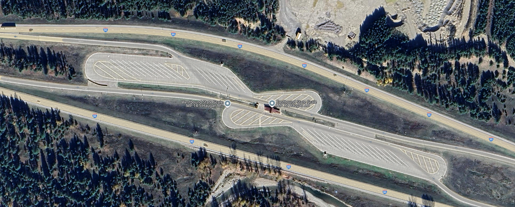
Overhead view of a median weigh station on I-90 in Haugan, Montana. Traffic from both eastbound and westbound lanes uses left exits to access the scales in the center. There are ample turnouts for parking trucks that fail one test or another. Source: Google Maps.
Most weigh stations in the US are located off the right side of the highway, as left-hand exit ramps are generally more dangerous than right exits. Still, a single weigh station located in the median of the highway can serve traffic from both directions, so the extra risk of accidents from exiting the highway to the left is often outweighed by the savings of not having to build two separate facilities. Either way, the main feature of a weigh station is the scale house, a building with large windows that offer a commanding view of the entire plaza as well as an up-close look at the trucks passing over the scales embedded in the pavement directly adjacent to the structure.
Scales at a weigh station are generally of two types: static scales, and weigh-in-motion (WIM) systems. A static scale is a large platform, called a weighbridge, set into a pit in the inspection lane, with the surface flush with the roadway. The platform floats within the pit, supported by a set of cantilevers that transmit the force exerted by the truck to electronic load cells. The signal from the load cells is cleaned up by signal conditioners before going to analog-to-digital converters and being summed and dampened by a scale controller in the scale house.
The weighbridge on a static scale is usually long enough to accommodate an entire semi tractor and trailer, which accurately weighs the entire vehicle in one measurement. The disadvantage is that the entire truck has to come to a complete stop on the weighbridge to take a measurement. Add in the time it takes for the induced motion of the weighbridge to settle, along with the time needed for the driver to make a slow approach to the scale, and each measurement can add up to significant delays for truckers.
Weigh-in-motion sensor. WIM systems measure the force exerted by each axle and calculate a total gross vehicle weight (GVW) for the truck while it passes over the sensor. The spacing between axles is also measured to ensure compliance with state laws. Source: Central Carolina Scales, Inc.
To avoid these issues, weigh-in-motion systems are often used. WIM systems use much the same equipment as the weighbridge on a static scale, although they tend to use piezoelectric sensors rather than traditional strain-gauge load cells, and usually have a platform that’s only big enough to have one axle bear on it at a time. A truck using a WIM scale remains in motion while the force exerted by each axle is measured, allowing the controller to come up with a final GVW as well as weights for each axle. While some WIM systems can measure the weight of a vehicle at highway speed, most weigh stations require trucks to keep their speed pretty slow, under five miles per hour. This is obviously for everyone’s safety, and even though the somewhat stately procession of trucks through a WIM can still plug traffic up, keeping trucks from having to come to a complete stop and set their brakes greatly increases weigh station throughput.
Another advantage of WIM systems is that the spacing between axles can be measured. The speed of the truck through the scale can be measured, usually using a pair of inductive loops embedded in the roadway around the WIM sensors. Knowing the vehicle’s speed through the scale allows the scale controller to calculate the distance between axles. Some states strictly regulate the distance between a trailer’s kingpin, which is where it attaches to the tractor, and the trailer’s first axle. Trailers that are not in compliance can be flagged and directed to a parking area to await a service truck to come by to adjust the spacing of the trailer bogie.
Keep It Moving, Buddy
A PrePass transponder reader and antenna over Interstate 10 near Pearlington, Mississippi. Trucks can bypass a weigh station if their in-cab transponder identifies them as certified. Source: Tony Webster, CC BY-SA 2.0.
Despite the increased throughput of WIM scales, there are often too many trucks trying to use a weigh station at peak times. To reduce congestion further, some states participate in automatic bypass systems. These systems, generically known as PrePass for the specific brand with the greatest market penetration, use in-cab transponders that are interrogated by transmitters mounted over the roadway well in advance of the weigh station. The transponder code is sent to PrePass for authentication, and if the truck ID comes back to a company that has gone through the PrePass certification process, a signal is sent to the transponder telling the driver to bypass the weigh station. The transponder lights a green LED in this case, which stays lit for about 15 minutes, just in case the driver gets stopped by an overzealous trooper who mistakes the truck for a scofflaw.
PrePass transponders are just one aspect of an entire suite of automatic vehicle identification (AVI) systems used in the typical modern weigh station. Most weigh stations are positively bristling with cameras, some of which are dedicated to automatic license plate recognition. These are integrated into the scale controller system and serve to associate WIM data with a specific truck, so violations can be flagged. They also help with the enforcement of traffic laws, as well as locating human traffickers, an increasingly common problem. Weigh stations also often have laser scanners mounted on bridges over the approach lanes to detect unpermitted oversized loads. Image analysis systems are also used to verify the presence and proper operation of required equipment, such a mirrors, lights, and mudflaps. Some weigh stations also have systems that can interrogate the electronic logging device inside the cab to verify that the driver isn’t in violation of hours of service laws, which dictate how long a driver can be on the road before taking breaks.
Sensors Galore
IR cameras watch for heat issues on trucks at a Kentucky weigh station. Heat signatures can be used to detect bad tires, stuck brakes, exhaust problems, and even illicit cargo. Source: Trucking Life with Shawn
Another set of sensors often found in the outer reaches of the weigh station plaza is related to the mechanical status of the truck. Infrared cameras are often used to scan for excessive heat being emitted by an axle, often a sign of worn or damaged brakes. The status of a truck’s tires can also be monitored thanks to Tire Anomaly and Classification Systems (TACS), which use in-road sensors that can analyze the contact patch of each tire while the vehicle is in motion. TACS can detect flat tires, over- and under-inflated tires, tires that are completely missing from an axle, or even mismatched tires. Any of these anomalies can cause a tire to quickly wear out and potentially self-destruct at highway speeds, resulting in catastrophic damage to surrounding traffic.
Trucks with problems are diverted by overhead signboards and direction arrows to inspection lanes. There, trained truck inspectors will closely examine the flagged problem and verify the violation. If the problem is relatively minor, like a tire inflation problem, the driver might be able to fix the issue and get back on the road quickly. Trucks that can’t be made safe immediately might have to wait for mobile service units to come fix the problem, or possibly even be taken off the road completely. Only after the vehicle is rendered road-worthy again can you keep on trucking.
We haven’t seen any projects from serial experimenter [Les Wright] for quite a while, and honestly, we were getting a little worried about that. Turns out we needn’t have fretted, as [Les] was deep into this exploration of the Pockels Effect, with pretty cool results.
If you’ll recall, [Les]’s last appearance on these pages concerned the automated creation of huge, perfect crystals of KDP, or potassium dihydrogen phosphate. KDP crystals have many interesting properties, but the focus here is on their ability to modulate light when an electrical charge is applied to the crystal. That’s the Pockels Effect, and while there are commercially available Pockels cells available for use mainly as optical switches, where’s the sport in buying when you can build?
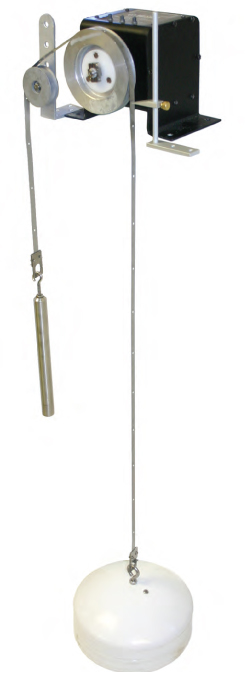
As with most of [Les]’s projects, there are hacks galore here, but the hackiest is probably the homemade diamond wire saw. The fragile KDP crystals need to be cut before use, and rather than risk his beauties to a bandsaw or angle grinder, [Les] threw together a rig using a stepper motor and some cheap diamond-encrusted wire. The motor moves the diamond wire up and down while a weight forces the crystal against it on a moving sled. Brilliant!
The cut crystals are then polished before being mounted between conductive ITO glass and connected to a high-voltage supply. The video below shows the beautiful polarization changes induced by the electric field, as well as demonstrating how well the Pockels cell acts as an optical switch. It’s kind of neat to see a clear crystal completely block a laser just by flipping a switch.
It’s an inconvenient fact that most of Earth’s largesse of useful minerals is locked up in, under, and around a lot of rock. Our little world condensed out of the remnants of stars whose death throes cooked up almost every element in the periodic table, and in the intervening billions of years, those elements have sorted themselves out into deposits that range from the easily accessed, lying-about-on-the-ground types to those buried deep in the crust, or worse yet, those that are distributed so sparsely within a mineral matrix that it takes harvesting megatonnes of material to find just a few kilos of the stuff.
Whatever the substance of our desires, and no matter how it is associated with the rocks and minerals below our feet, almost every mining and refining effort starts with wresting vast quantities of rock from the Earth’s crust. And the easiest, cheapest, and fastest way to do that most often involves blasting. In a very real way, explosives make the world work, for without them, the minerals we need to do almost anything would be prohibitively expensive to produce, if it were possible at all. And understanding the chemistry, physics, and engineering behind blasting operations is key to understanding almost everything about Mining and Refining.
First, We Drill
For almost all of the time that we’ve been mining minerals, making big rocks into smaller rocks has been the work of strong backs and arms supplemented by the mechanical advantage of tools like picks, pry bars, and shovels. The historical record shows that early miners tried to reduce this effort with clever applications of low-energy physics, such as jamming wooden plugs into holes in the rocks and soaking them with liquid to swell the wood and exert enough force to fracture the rock, or by heating the rock with bonfires and then flooding with cold water to create thermal stress fractures. These methods, while effective, only traded effort for time, and only worked for certain types of rock.
Mining productivity got a much-needed boost in 1627 with the first recorded use of gunpowder for blasting at a gold mine in what is now Slovakia. Boreholes were stuffed with powder that was ignited by a fuse made from a powder-filled reed. The result was a pile of rubble that would have taken weeks to produce by hand, and while the speed with which the explosion achieved that result was probably much welcomed by the miners, in reality, it only shifted their efforts to drilling the boreholes, which generally took a five-man crew using sledgehammers and striker bars to pound deep holes into the rock. Replacing that manual effort with mechanical drilling was the next big advance, but it would have to wait until the Industrial Revolution harnessed the power of steam to run drills capable of boring deep holes in rock quickly and with much smaller crews.
The basic principles of rock drilling developed in the 19th century, such as rapidly spinning a hardened steel bit while exerting tremendous down-pressure and high-impulse percussion, remain applicable today, although with advancements like synthetic diamond tooling and better methods of power transmission. Modern drills for open-cast mining fall into two broad categories: overburden drills, which typically drill straight down or at a slight angle to vertical and can drill large-diameter holes over 100 meters deep, and quarry drills, which are smaller and more maneuverable rigs that can drill at any angle, even horizontally. Most drill rigs are track-driven for greater mobility over rubble-strewn surfaces, and are equipped with soundproofed, air-conditioned cabs with safety cages to protect the operator. Automation is a big part of modern rigs, with automatic leveling systems, tool changers that can select the proper bit for the rock type, and fully automated drill chain handling, including addition of drill rod to push the bit deeper into the rock. Many drill rigs even have semi-autonomous operation, where a single operator can control a fleet of rigs from a single remote control console.
Proper Prior Planning
While the use of explosives seems brutally chaotic and indiscriminate, it’s really the exact opposite. Each of the so-called “shots” in a blasting operation is a carefully controlled, highly engineered event designed to move material in a specific direction with the desired degree of fracturing, all while ensuring the safety of the miners and the facility.
To accomplish this, a blasting plan is put together by a mining engineer. The blasting plan takes into account the mechanical characteristics of the rock, the location and direction of any pre-existing fractures or faults, and proximity to any structures or hazards. Engineers also need to account for the equipment used for mucking, which is the process of removing blasted material for further processing. For instance, a wheeled loader operating on the same level, or bench, that the blasting took place on needs a different size and shape of rubble pile than an excavator or dragline operating from the bench above. The capabilities of the rock crushing machinery that’s going to be used to process the rubble also have to be accounted for in the blasting plan.
Most blasting plans define a matrix of drill holes with very specific spacing, generally with long rows and short columns. The drill plan specifies the diameter of each hole along with its depth, which usually goes a little beyond the distance to the next bench down. The mining engineer also specifies a stem height for the hole, which leaves room on top of the explosives to backfill the hole with drill tailings or gravel.
Prills and Oil
Once the drill holes are complete and inspected, charging the holes with explosives can begin. The type of blasting agents to be used is determined by the blasting plan, but in most cases, the agent of choice is ANFO, or ammonium nitrate and fuel oil. The ammonium nitrate, which contains 60% oxygen by weight, serves as an oxidizer for the combustion of the long-chain alkanes in the fuel oil. The ideal mix is 94% ammonium nitrate to 6% fuel oil.
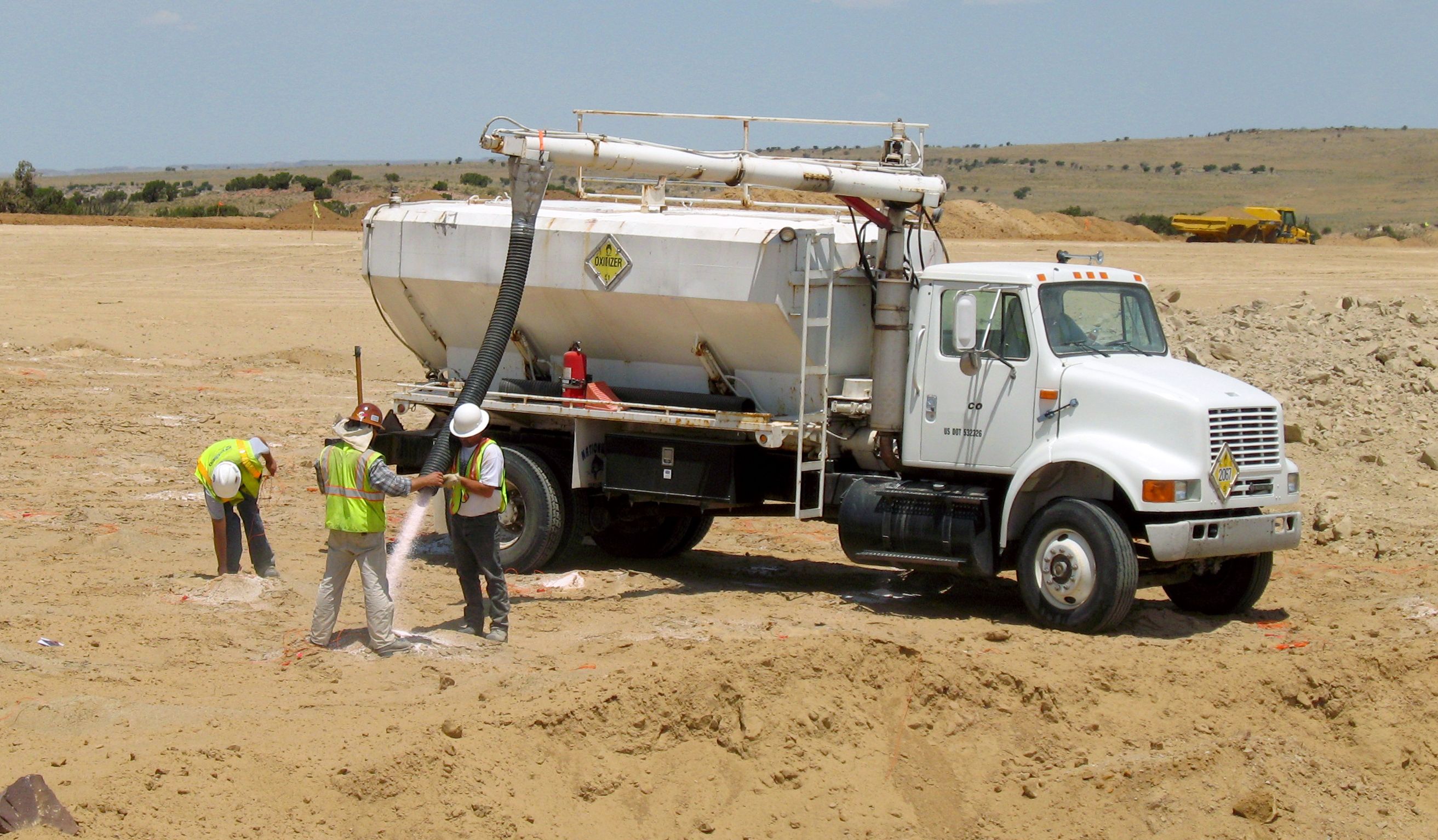
Filling holes with ammonium nitrate at a blasting site. Hopper trucks like this are often used to carry prilled ammonium nitrate. Some trucks also have a tank for the fuel oil that’s added to the ammonium nitrate to make ANFO. Credit: Old Bear Photo, via Adobe Stock.
How the ANFO is added to the hole depends on conditions. For holes where groundwater is not a problem, ammonium nitrate in the form of small porous beads or prills, is poured down the hole and lightly tamped to remove any voids or air spaces before the correct amount of fuel oil is added. For wet conditions, an ammonium nitrate emulsion will be used instead. This is just a solution of ammonium nitrate in water with emulsifiers added to allow the fuel oil to mix with the oxidizer.
ANFO is classified as a tertiary explosive, meaning it is insensitive to shock and requires a booster to detonate. The booster charge is generally a secondary explosive such as PETN, or pentaerythritol tetranitrate, a powerful explosive that’s chemically similar to nitroglycerine but is much more stable. PETN comes in a number of forms, with cardboard cylinders like oversized fireworks or a PETN-laced gel stuffed into a plastic tube that looks like a sausage being the most common.
Electrically operated blasting caps marked with their built-in 425 ms delay. These will easily blow your hand clean off. Source: Timo Halén, CC BY-SA 2.5.
Being a secondary explosive, the booster charge needs a fairly strong shock to detonate. This shock is provided by a blasting cap or detonator, which is a small, multi-stage pyrotechnic device. These are generally in the form of a small brass or copper tube filled with a layer of primary explosive such as lead azide or fulminate of mercury, along with a small amount of secondary explosive such as PETN. The primary charge is in physical contact with an initiator of some sort, either a bridge wire in the case of electrically initiated detonators, or more commonly, a shock tube. Shock tubes are thin-walled plastic tubing with a layer of reactive explosive powder on the inner wall. The explosive powder is engineered to detonate down the tube at around 2,000 m/s, carrying a shock wave into the detonator at a known rate, which makes propagation delays easy to calculate.
Timing is critical to the blasting plan. If the explosives in each hole were to all detonate at the same time, there wouldn’t be anywhere for the displaced material to go. To prevent that, mining engineers build delays into the blasting plan so that some charges, typically the ones closest to the free face of the bench, go off a fraction of a second before the charges behind them, freeing up space for the displaced material to move into. Delays are either built into the initiator as a layer of pyrotechnic material that burns at a known rate between the initiator and the primary charge, or by using surface delays, which are devices with fixed delays that connect the initiator down the hole to the rest of the charges that will make up the shot. Lately, electronic detonators have been introduced, which have microcontrollers built in. These detonators are addressable and can have a specific delay programmed in the field, making it easier to program the delays needed for the entire shot. Electronic detonators also require a specific code to be transmitted to detonate, which reduces the chance of injury or misuse that lost or stolen electrical blasting caps present. This was enough of a problem that a series of public service films on the dangers of playing with blasting caps appeared regularly from the 1950s through the 1970s.
“Fire in the Hole!”
When all the holes are charged and properly stemmed, the blasting crew makes the final connections on the surface. Connections can be made with wires for electrical and electronic detonators, or with shock tubes for non-electric detonators. Sometimes, detonating cord is used to make the surface connections between holes. Det cord is similar to shock tube but generally looks like woven nylon cord. It also detonates at a much faster rate (6,500 m/s) than shock tube thanks to being filled with PETN or a similar high-velocity explosive.
Once the final connections to the blasting controller are made and tested, the area is secured with all personnel and equipment removed. A series of increasingly urgent warnings are sounded on sirens or horns as the blast approaches, to alert personnel to the danger. The blaster initiates the shot at the controller, which sends the signal down trunklines and into any surface delays before being transmitted to the detonators via their downlines. The relatively weak shock wave from the detonator propagates into the booster charge, which imparts enough energy into the ANFO to start detonation of the main charge.
The ANFO rapidly decomposes into a mixture of hot gases, including carbon dioxide, nitrogen, and water vapor. The shock wave pulverizes the rock surrounding the borehole and rapidly propagates into the surrounding rock, exerting tremendous compressive force. The shock wave continues to propagate until it meets a natural crack or the interface between rock and air at the free face of the shot. These impedance discontinuities reflect the compressive wave and turn it into a tensile wave, and since rock is generally much weaker in tension than compression, this is where the real destruction begins.
The reflected tensile forces break the rock along natural or newly formed cracks, creating voids that are filled with the rapidly expanding gases from the burning ANFO. The gases force these cracks apart, providing the heave needed to move rock fragments into the voids created by the initial shock wave. The shot progresses at the set delay intervals between holes, with the initial shock from new explosions creating more fractures deeper into the rock face and more expanding gas to move the fragments into the space created by earlier explosions. Depending on how many holes are in the shot and how long the delays are, the entire thing can be over in just a few seconds, or it could go on for quite some time, as it does in this world-record blast at a coal mine in Queensland in 2019, which used 3,899 boreholes packed with 2,194 tonnes of ANFO to move 4.7 million cubic meters of material in just 16 seconds.
There’s still much for the blasting crew to do once the shot is done. As the dust settles, safety crews use monitoring equipment to ensure any hazardous blasting gases have dispersed before sending in crews to look for any misfires. Misfires can result in a reshoot, where crews hook up a fresh initiator and try to detonate the booster charge again. If the charge won’t fire, it can be carefully extracted from the rubble pile with non-sparking tools and soaked in water to inactivate it.
Hold onto your hats, everyone — there’s stunning news afoot. It’s hard to believe, but it looks like over-reliance on chatbots to do your homework can turn your brain into pudding. At least that seems to be the conclusion of a preprint paper out of the MIT Media Lab, which looked at 54 adults between the ages of 18 and 39, who were tasked with writing a series of essays. They divided participants into three groups — one that used ChatGPT to help write the essays, one that was limited to using only Google search, and one that had to do everything the old-fashioned way. They recorded the brain activity of writers using EEG, in order to get an idea of brain engagement with the task. The brain-only group had the greatest engagement, which stayed consistently high throughout the series, while the ChatGPT group had the least. More alarmingly, the engagement for the chatbot group went down even further with each essay written. The ChatGPT group produced essays that were very similar between writers and were judged “soulless” by two English teachers. Go figure.
The most interesting finding, though, was when 18 participants from the chatbot and brain-only groups were asked to rewrite one of their earlier essays, with the added twist that the chatbot group had to do it all by themselves, while the brainiacs got to use ChatGPT. The EEGs showed that the first group struggled with the task, presumably because they failed to form any deep memory of their previous work thanks to over-reliance on ChatGPT. The brain-only folks, however, did well at the task and showed signs of activity across all EEG bands. That fits well with our experience with chatbots, which we use to help retrieve specific facts and figures while writing articles, especially ones we know we’ve seen during our initial scan of the literature but can’t find later.
Does anyone remember Elektro? We sure do, although not from personal experience, since the seven-foot-tall automaton built by Westinghouse for the World’s Fair in New York City in 1939 significantly predates our appearance on the planet. But still, the golden-skinned robot that made its living by walking around, smoking, and cracking wise at the audience thanks to a 78-rpm record player in its capacious chest, really made an impression, enough that it toured the country for the better part of 30 years and made the unforgettable Sex Kittens Go to College in 1960 before fading into obscurity. At some point, the one-of-a-kind robot was rescued from a scrap heap and restored to its former glory, and now resides in the North Central Ohio Industrial Museum in Mansfield, very close to the Westinghouse facility that built it. If you need an excuse to visit North Central Ohio, you could do worse than a visit to see Elektro.
It was with some alarm that we learned this week from Al Williams that mtrek.com 1701 appeared to be down. For those not in the know, mtrek is a Telnet space combat game inspired by the Star Trek franchise, which explains why Al was in such a tizzy about not being able to connect; huge Trek nerd, our Al. Anyway, it appears Al’s worst fears were unfounded, as we were able to connect to mtrek just fine. But in the process of doing so, we stumbled across this collection of Telnet games and demos that’s worth checking out. The mtrek, of course, as well as Telnet versions of chess and backgammon, and an interactive world map that always blows our mind. The site also lists the Telnet GOAT, the Star Wars Asciimation; sadly, that one does seem to be down, at least for us. Sure, you can see it in a web browser, but it’s not the same as watching it in a terminal over Telnet, is it?
And finally, if you’ve got 90 minutes or so to spare, you could do worse than to spend it with our friend Hash as he reverse engineers an automotive ECU. We have to admit that we haven’t indulged yet — it’s on our playlist for this weekend, because we know how to party. But from what Hash tells us, this is the tortured tale of a job that took far, far longer to complete than expected. We have to admit that while we’ll gladly undertake almost any mechanical repair on most vehicles, automotive ECUs and other electronic modules are almost a bridge too far for us, at least in terms of cracking them open to make even simple repairs. Getting access to them for firmware extraction and parameter fiddling sounds like a lot of fun, and we’re looking forward to hearing what Hash has to say about the subject.
For a world covered in oceans, getting a drink of water on Planet Earth can be surprisingly tricky. Fresh water is hard to come by even on our water world, so much so that most sources are better measured in parts per million than percentages; add together every freshwater lake, river, and stream in the world, and you’d be looking at a mere 0.0066% of all the water on Earth.
Of course, what that really says is that our endowment of saltwater is truly staggering. We have over 1.3 billion cubic kilometers of the stuff, most of it easily accessible to the billion or so people who live within 10 kilometers of a coastline. Untreated, though, saltwater isn’t of much direct use to humans, since we, our domestic animals, and pretty much all our crops thirst only for water a hundred times less saline than seawater.
While nature solved the problem of desalination a long time ago, the natural water cycle turns seawater into freshwater at too slow a pace or in the wrong locations for our needs. While there are simple methods for getting the salt out of seawater, such as distillation, processing seawater on a scale that can provide even a medium-sized city with a steady source of potable water is definitely a job for Big Chemistry.
Biology Backwards
Understanding an industrial chemistry process often starts with a look at the feedstock, so what exactly is seawater? It seems pretty obvious, but seawater is actually a fairly complex solution that varies widely in composition. Seawater averages about 3.5% salinity, which means there are 35 grams of dissolved salts in every liter. The primary salt is sodium chloride, with potassium, magnesium, and calcium salts each making a tiny contribution to the overall salinity. But for purposes of acting as a feedstock for desalination, seawater can be considered a simple sodium chloride solution where sodium anions and chloride cations are almost completely dissociated. The goal of desalination is to remove those ions, leaving nothing but water behind.
While thermal desalination methods, such as distillation, are possible, they tend not to scale well to industrial levels. Thermal methods have their place, though, especially for shipboard potable water production and in cases where fuel is abundant or solar energy can be employed to heat the seawater directly. However, in most cases, industrial desalination is typically accomplished through reverse osmosis RO, which is the focus of this discussion.
In biological systems, osmosis is the process by which cells maintain equilibrium in terms of concentration of solutes relative to the environment. The classic example is red blood cells, which if placed in distilled water will quickly burst. That’s because water from the environment, which has a low concentration of solutes, rushes across the semi-permeable cell membrane in an attempt to dilute the solutes inside the cell. All that water rushing into the cell swells it until the membrane can’t take the pressure, resulting in hemolysis. Conversely, a blood cell dropped into a concentrated salt solution will shrink and wrinkle, or crenellate, as the water inside rushes out to dilute the outside environment.
Water rushes in, water rushes out. Either way, osmosis is bad news for red blood cells. Reversing the natural osmotic flow of a solution like seawater is the key to desalination by reverse osmosis. Source: Emekadecatalyst, CC BY-SA 4.0.
Reverse osmosis is the opposite process. Rather than water naturally following a concentration gradient to equilibrium, reverse osmosis applies energy in the form of pressure to force the water molecules in a saline solution through a semipermeable membrane, leaving behind as many of the salts as possible. What exactly happens at the membrane to sort out the salt from the water is really the story, and as it turns out, we’re still not completely clear how reverse osmosis works, even though we’ve been using it to process seawater since the 1950s.
Battling Models
Up until the early 2020s, the predominant model for how reverse osmosis (RO) worked was called the “solution-diffusion” model. The SD model treated RO membranes as effectively solid barriers through which water molecules could only pass by first diffusing into the membrane from the side with the higher solute concentration. Once inside the membrane, water molecules would continue through to the other side, the permeate side, driven by a concentration gradient within the membrane. This model had several problems, but the math worked well enough to allow the construction of large-scale seawater RO plants.
The new model is called the “solution-friction” model, and it better describes what’s going on inside the membrane. Rather than seeing the membrane as a solid barrier, the SF model considers the concentrate and permeate surfaces of the membrane to communicate through a series of interconnected pores. Water is driven across the membrane not by concentration but by a pressure gradient, which drives clusters of water molecules through the pores. The friction of these clusters against the walls of the pores results in a linear pressure drop across the membrane, an effect that can be measured in the lab and for which the older SD model has no explanation.
As for the solutes in a saline solution, the SF model accounts for their exclusion from the permeate by a combination of steric hindrance (the solutes just can’t fit through the pores), the Donnan effect (which says that ions with the opposite charge of the membrane will get stuck inside it), and dielectric exclusion (the membrane presents an energy barrier that makes it hard for ions to enter it). The net result of these effects is that ions tend to get left on one side of the membrane, while water molecules can squeeze through more easily to the permeate side.
Turning these models into a practical industrial process takes a great deal of engineering. A seawater reverse osmosis or SWRO, plant obviously needs to be located close to the shore, but also needs to be close to supporting infrastructure such as a municipal water system to accept the finished product. SWRO plants also use a lot of energy, so ready access to the electrical grid is a must, as is access to shipping for the chemicals needed for pre- and post-treatment.
Pores and Pressure
Seawater processing starts with water intake. Some SWRO plants use open intakes located some distance out from the shoreline, well below the lowest possible tides and far from any potential source of contamination or damage, such a ship anchorages. Open intakes generally have grates over them to exclude large marine life and debris from entering the system. Other SWRO plants use beach well intakes, with shafts dug into the beach that extend below the water table. Seawater filters through the sand and fills the well; from there, the water is pumped into the plant. Beach wells have the advantage of using the beach sand as a natural filter for particulates and smaller sea critters, but do tend to have a lower capacity than open intakes.
Aside from the salts, seawater has plenty of other unwanted bits, all of which need to come out prior to reverse osmosis. Trash racks remove any shells, sea life, or litter that manage to get through the intakes, and sand bed filters are often used to remove smaller particulates. Ultrafiltration can be used to further clarify the seawater, and chemicals such as mild acids or bases are often used to dissolve inorganic scale and biofilms. Surfactants are often added to the feedstock, too, to break up heavy organic materials.
By the time pretreatment is complete, the seawater is remarkably free from suspended particulates and silt. Pretreatment aims to reduce the turbidity of the feedstock to less than 0.5 NTUs, or nephelometric turbidity units. For context, the US Environmental Protection Agency standard for drinking water is 0.3 NTUs for 95% of the samples taken in a month. So the pretreated seawater is almost as clear as drinking water before it goes to reverse osmosis.
SWRO cartridges have membranes wound into spirals and housed in pressure vessels. Seawater under high pressure enters the membrane spiral; water molecules migrate across the membrane to a center permeate tube, leaving a reject brine that’s about twice as saline as the feedstock. Source: DuPont Water Solutions.
The heart of reverse osmosis is the membrane, and a lot of engineering goes into it. Modern RO membranes are triple-layer thin-film composites that start with a non-woven polyester support, a felt-like material that provides the mechanical strength to withstand the extreme pressures of reverse osmosis. Next comes a porous support layer, a 50 μm-thick layer of polysulfone cast directly onto the backing layer. This layer adds to the physical strength of the backing and provides a strong yet porous foundation for the active layer, a cross-linked polyamide layer about 100 to 200 nm thick. This layer is formed by interfacial polymerization, where a thin layer of liquid monomer and initiators is poured onto the polysulfone to polymerize in place.
An RO rack in a modern SWRO desalination plant. Each of the white tubes is a pressure vessel containing seven or eight RO membrane cartridges. The vessels are plumbed in parallel to increase flow through the system. Credit: Elvis Santana, via Adobe Stock.
Modern membranes can flow about 35 liters per square meter every hour, which means an SWRO plant needs to cram a lot of surface area into a little space. This is accomplished by rolling the membrane up into a spiral and inserting it into a fiberglass pressure vessel, which holds seven or eight cartridges. Seawater pumped into the vessel soaks into the backing layer to the active layer, where only the water molecules pass through and into a collection pipe at the center of the roll. The desalinated water, or permeate, exits the cartridge through the center pipe while rejected brine exits at the other end of the pressure vessel.
The pressure needed for SWRO is enormous. The natural osmotic pressure of seawater is about 27 bar (27,000 kPa), which is the pressure needed to halt the natural flow of water across a semipermeable membrane. SWRO systems must pressurize the water to at least that much plus a net driving pressure (NPD) to overcome mechanical resistance to flow through the membrane, which amounts to an additional 30 to 40 bar.
Energy Recovery
To achieve these tremendous pressures, SWRO plants use multistage centrifugal pumps driven by large, powerful electric motors, often 300 horsepower or more for large systems. The electricity needed to run those motors accounts for 60 to 80 percent of the energy costs of the typical SWRO plant, so a lot of effort is put into recovering that energy, most of which is still locked up in the high-pressure rejected brine as hydraulic energy. This energy used to be extracted by Pelton-style turbines connected to the shaft of the main pressure pump; the high-pressure brine would spin the pump shaft and reduce the mechanical load on the pump, which would reduce the electrical load. Later, the brine’s energy would be recovered by a separate turbo pump, which would boost the pressure of the feed water before it entered the main pump.
While both of these methods were capable of recovering a large percentage of the input energy, they were mechanically complex. Modern SWRO plants have mostly moved to isobaric energy recovery devices, which are mechanically simpler and require much less maintenance. Isobaric ERDs have a single moving part, a cylindrical ceramic rotor. The rotor has a series of axial holes, a little like the cylinder of an old six-shooter revolver. The rotor is inside a cylindrical housing with endcaps on each end, each with an inlet and an outlet fitting. High-pressure reject brine enters the ERD on one side while low-pressure seawater enters on the other side. The slugs of water fill the same bore in the rotor and equalize at the same pressure without much mixing thanks to the different densities of the fluids. The rotor rotates thanks to the momentum carried by the incoming water streams and inlet fittings that are slightly angled relative to the axis of the bore. When the rotor lines up with the outlet fittings in each end cap, the feed water and the brine both exit the rotor, with the feed water at a higher pressure thanks to the energy of the reject brine.
For something with only one moving part, isobaric ERDs are remarkably effective. They can extract about 98% of the energy in the reject brine, pressuring the feed water about 60% of the total needed. An SWRO plant with ERDs typically uses 5 to 6 kWh to produce a cubic meter of desalinated water; ERDs can slash that to just 2 to 3 kWh.
Isobaric energy recovery devices can recover half of the electricity used by the typical SWRO plant by using the pressure of the reject brine to pressurize the feed water. Source: Flowserve.
Finishing Up
Once the rejected brine’s energy has been recovered, it needs to be disposed of properly. This is generally done by pumping it back out into the ocean through a pipe buried in the seafloor. The outlet is located a considerable distance from the inlet and away from any ecologically sensitive areas. The brine outlet is also generally fitted with a venturi induction head, which entrains seawater from around the outlet to partially dilute the brine.
As for the permeate that comes off the RO racks, while it is almost completely desalinated and very clean, it’s still not suitable for distribution into the drinking water system. Water this clean is highly corrosive to plumbing fixtures and has an unpleasantly flat taste. To correct this, RO water is post-processed by passing it over beds of limestone chips. The RO water tends to be slightly acidic thanks to dissolved CO2, so it partially dissolves the calcium carbonate in the limestone. This raises the pH closer to neutral and adds calcium ions to the water, which increases its hardness a bit. The water also gets a final disinfection with chlorine before being released to the distribution network.
Are robotaxis poised to be the Next Big Thing in North America? It seems so, at least according to Goldman Sachs, which issued a report this week stating that robotaxis have officially entered the commercialization phase of the hype cycle. That assessment appears to be based on an analysis of the total ride-sharing market, which encompasses services that are currently almost 100% reliant on meat-based drivers, such as Lyft and Uber, and is valued at $58 billion. Autonomous ride-hailing services like Waymo, which has a fleet of 1,500 robotaxis operating in several cities across the US, are included in that market but account for less than 1% of the total right now. But, Goldman projects that the market will burgeon to over $336 billion in the next five years, driven in large part by “hyperscaling” of autonomous vehicles.
We suspect the upcoming launch of Tesla’s robotaxis in Austin, Texas, accounts for some of this enthusiasm for the near-term, but we have our doubts that a market based on such new and complex technologies can scale that quickly. A little back-of-the-envelope math suggests that the robotaxi fleet will need to grow to about 9,000 cars in the next five years, assuming the same proportion of autonomous cars in the total ride-sharing fleet as exists today. A look inside the Waymo robotaxi plant outside of Phoenix reveals that it can currently only convert “several” Jaguar electric SUVs per day, meaning they’ve got a lot of work to do to meet the needed numbers. Other manufacturers will no doubt pitch in, especially Tesla, and factory automation always seems to pull off miracles under difficult circumstances, but it still seems like a stretch to think there’ll be that many robotaxis on the road in only five years. Also, it currently costs more to hail a robotaxi than an Uber or Lyft, and we just don’t see why anyone would prefer to call a robotaxi, unless it’s for the novelty of the experience.
On the other hand, if the autonomous ride-sharing market does experience explosive growth, there could be knock-on benefits even for Luddite naysayers such as we. A report, again from Goldman Sachs — hey, they probably have a lot of skin in the game — predicts that auto insurance rates could fall by 50% as more autonomous cars hit the streets. This is based on markedly lower liability for self-driving cars, which have 92% fewer bodily injury claims and 88% lower property damage claims than human-driven cars. Granted, those numbers have to be based on a very limited population, and we guarantee that self-drivers will find new and interesting ways to screw up on the road. But if our insurance rates fall even a little because of self-driving cars, we’ll take it as a win.
Speaking of robotics, if you want to see just how far we’ve come in terms of robot dexterity, look no further than the package-sorting abilities of Figure’s Helix robot. The video in the article is an hour long, but you don’t need to watch more than a few minutes to be thoroughly impressed. The robot is standing at a sorting table with an infeed conveyor loaded with just about the worst parcels possible, a mix of soft, floppy, poly-bagged packages, flat envelopes, and traditional boxes. The robot was tasked with placing the parcels on an outfeed conveyor, barcode-side down, and with proper separation between packages. It also treats the soft poly-bag parcels to a bit of extra attention, pressing them down a bit to flatten them before flicking them onto the belt. Actually, it’s that flicking action that seems the most human, since it’s accompanied by a head-swivel to the infeed belt to select its next package. Assuming this is legit autonomous and not covertly teleoperated, which we have no reason to believe, the manual dexterity on display here is next-level; we’re especially charmed by the carefree little package flip about a minute in. The way it handles mistakenly grabbing two packages at once is pretty amazing, too.
And finally, our friend Leo Fernekes dropped a new video that’ll hit close to home for a lot of you out there. Leo is a bit of a techno-hoarder, you see, and with the need to make some room at home and maintain his domestic tranquility, he had to tackle the difficult process of getting rid of old projects, some of which date back 40 or more years. Aside from the fun look through his back-catalog of projects, the video is also an examination of the emotional attachments we hackers tend to develop to our projects. We touched on that a bit in our article on tech anthropomorphization, but we see how going through these projects is not only a snapshot of the state of the technology available at the time, but also a slice of life. Each of the projects is not just a collection of parts, they’re collections of memories of where Leo was in life at the time. Sometimes it’s hard to let go of things that are so strongly symbolic of a time that’s never coming back, and we applaud Leo for having the strength to pitch that stuff. Although seeing a clock filled with 80s TTL chips and a vintage 8085 microprocessor go into the bin was a little tough to watch.
What happens when you build the largest machine in the world, but it’s still not big enough? That’s the situation the North American transmission system, the grid that connects power plants to substations and the distribution system, and which by some measures is the largest machine ever constructed, finds itself in right now. After more than a century of build-out, the towers and wires that stitch together a continent-sized grid aren’t up to the task they were designed for, and that’s a huge problem for a society with a seemingly insatiable need for more electricity.
There are plenty of reasons for this burgeoning demand, including the rapid growth of data centers to support AI and other cloud services and the move to wind and solar energy as the push to decarbonize the grid proceeds. The former introduces massive new loads to the grid with millions of hungry little GPUs, while the latter increases the supply side, as wind and solar plants are often located out of reach of existing transmission lines. Add in the anticipated expansion of the manufacturing base as industry seeks to re-home factories, and the scale of the potential problem only grows.
The bottom line to all this is that the grid needs to grow to support all this growth, and while there is often no other solution than building new transmission lines, that’s not always feasible. Even when it is, the process can take decades. What’s needed is a quick win, a way to increase the capacity of the existing infrastructure without having to build new lines from the ground up. That’s exactly what reconductoring promises, and the way it gets there presents some interesting engineering challenges and opportunities.
Bare Metal
Copper is probably the first material that comes to mind when thinking about electrical conductors. Copper is the best conductor of electricity after silver, it’s commonly available and relatively easy to extract, and it has all the physical characteristics, such as ductility and tensile strength, that make it easy to form into wire. Copper has become the go-to material for wiring residential and commercial structures, and even in industrial installations, copper wiring is a mainstay.
However, despite its advantages behind the meter, copper is rarely, if ever, used for overhead wiring in transmission and distribution systems. Instead, aluminum is favored for these systems, mainly due to its lower cost compared to the equivalent copper conductor. There’s also the factor of weight; copper is much denser than aluminum, so a transmission system built on copper wires would have to use much sturdier towers and poles to loft the wires. Copper is also much more subject to corrosion than aluminum, an important consideration for wires that will be exposed to the elements for decades.
ACSR (left) has a seven-strand steel core surrounded by 26 aluminum conductors in two layers. ACCC has three layers of trapezoidal wire wrapped around a composite carbon fiber core. Note the vastly denser packing ratio in the ACCC. Source: Dave Bryant, CC BY-SA 3.0.
Aluminum has its downsides, of course. Pure aluminum is only about 61% as conductive as copper, meaning that conductors need to have a larger circular area to carry the same amount of current as a copper cable. Aluminum also has only about half the tensile strength of copper, which would seem to be a problem for wires strung between poles or towers under a lot of tension. However, the greater diameter of aluminum conductors tends to make up for that lack of strength, as does the fact that most aluminum conductors in the transmission system are of composite construction.
The vast majority of the wires in the North American transmission system are composites of aluminum and steel known as ACSR, or aluminum conductor steel-reinforced. ACSR is made by wrapping high-purity aluminum wires around a core of galvanized steel wires. The core can be a single steel wire, but more commonly it’s made from seven strands, six wrapped around a single central wire; especially large ACSR might have a 19-wire core. The core wires are classified by their tensile strength and the thickness of their zinc coating, which determines how corrosion-resistant the core will be.
In standard ACSR, both the steel core and the aluminum outer strands are round in cross-section. Each layer of the cable is twisted in the opposite direction from the previous layer. Alternating the twist of each layer ensures that the finished cable doesn’t have a tendency to coil and kink during installation. In North America, all ACSR is constructed so that the outside layer has a right-hand lay.
ACSR is manufactured by machines called spinning or stranding machines, which have large cylindrical bodies that can carry up to 36 spools of aluminum wire. The wires are fed from the spools into circular spinning plates that collate the wires and spin them around the steel core fed through the center of the machine. The output of one spinning frame can be spooled up as finished ACSR or, if more layers are needed, can pass directly into another spinning frame for another layer of aluminum, in the opposite direction, of course.
Fiber to the Core
While ACSR is the backbone of the grid, it’s not the only show in town. There’s an entire beastiary of initialisms based on the materials and methods used to build composite cables. ACSS, or aluminum conductor steel-supported, is similar to ACSR but uses more steel in the core and is completely supported by the steel, as opposed to ACSR where the load is split between the steel and the aluminum. AAAC, or all-aluminum alloy conductor, has no steel in it at all, instead relying on high-strength aluminum alloys for the necessary tensile strength. AAAC has the advantage of being very lightweight as well as being much more resistant to core corrosion than ACSR.
Another approach to reducing core corrosion for aluminum-clad conductors is to switch to composite cores. These are known by various trade names, such as ACCC (aluminum conductor composite core) or ACCR (aluminum conductor composite reinforced). In general, these cables are known as HTLS, which stands for high-temperature, low-sag. They deliver on these twin promises by replacing the traditional steel core with a composite material such as carbon fiber, or in the case of ACCR, a fiber-reinforced metal matrix.
The point of composite cores is to provide the conductor with the necessary tensile strength and lower thermal expansion coefficient, so that heating due to loading and environmental conditions causes the cable to sag less. Controlling sag is critical to cable capacity; the less likely a cable is to sag when heated, the more load it can carry. Additionally, composite cores can have a smaller cross-sectional area than a steel core with the same tensile strength, leaving room for more aluminum in the outer layers while maintaining the same overall conductor diameter. And of course, more aluminum means these advanced conductors can carry more current.
Another way to increase the capacity in advanced conductors is by switching to trapezoidal wires. Traditional ACSR with round wires in the core and conductor layers has a significant amount of dielectric space trapped within the conductor, which contributes nothing to the cable’s current-carrying capacity. Filling those internal voids with aluminum is accomplished by wrapping round composite cores with aluminum wires that have a trapezoidal cross-section to pack tightly against each other. This greatly reduces the dielectric space trapped within a conductor, increasing its ampacity within the same overall diameter.
Unfortunately, trapezoidal aluminum conductors are much harder to manufacture than traditional round wires. While creating the trapezoids isn’t that much harder than drawing round aluminum wire — it really just requires switching to a different die — dealing with non-round wire is more of a challenge. Care must be taken not to twist the wire while it’s being rolled onto its spools, as well as when wrapping the wire onto the core. Also, the different layers of aluminum in the cable require different trapezoidal shapes, lest dielectric voids be introduced. The twist of the different layers of aluminum has to be controlled, too, just as with round wires. Trapezoidal wires can also complicate things for linemen in the field in terms of splicing and terminating cables, although most utilities and cable construction companies have invested in specialized tooling for advanced conductors.
Same Towers, Better Wires
The grid is what it is today in large part because of decisions made a hundred or more years ago, many of which had little to do with engineering. Power plants were located where it made sense to build them relative to the cities and towns they would serve and the availability of the fuel that would power them, while the transmission lines that move bulk power were built where it was possible to obtain rights-of-way. These decisions shaped the physical footprint of the grid, and except in cases where enough forethought was employed to secure rights-of-way generous enough to allow for expansion of the physical plant, that footprint is pretty much what engineers have to work with today.
Increasing the amount of power that can be moved within that limited footprint is what reconductoring is all about. Generally, reconductoring is pretty much what it sounds like: replacing the conductors on existing support structures with advanced conductors. There are certainly cases where reconductoring alone won’t do, such as when new solar or wind plants are built without existing transmission lines to connect them to the system. In those cases, little can be done except to build a new transmission line. And even where reconductoring can be done, it’s not cheap; it can cost 20% more per mile than building new towers on new rights-of-way. But reconductoring is much, much faster than building new lines. A typical reconductoring project can be completed in 18 to 36 months, as compared to the 5 to 15 years needed to build a new line, thanks to all the regulatory and legal challenges involved in obtaining the property to build the structures on. Reconductoring usually faces fewer of these challenges, since rights-of-way on existing lines were established long ago.
The exact methods of reconductoring depend on the specifics of the transmission line, but in general, reconductoring starts with a thorough engineering evaluation of the support structures. Since most advanced conductors are the same weight per unit length as the ACSR they’ll be replacing, loads on the towers should be about the same. But it’s prudent to make sure, and a field inspection of the towers on the line is needed to make sure they’re up to snuff. A careful analysis of the design capacity of the new line is also performed before the project goes through the permitting process. Reconductoring is generally performed on de-energized lines, which means loads have to be temporarily shifted to other lines, requiring careful coordination between utilities and transmission operators.
Once the preliminaries are in place, work begins. Despite how it may appear, most transmission lines are not one long cable per phase that spans dozens of towers across the countryside. Rather, most lines span just a few towers before dead-ending into insulators that use jumpers to carry current across to the next span of cable. This makes reconductoring largely a tower-by-tower affair, which somewhat simplifies the process, especially in terms of maintaining the tension on the towers while the conductors are swapped. Portable tensioning machines are used for that job, as well as for setting the proper tension in the new cable, which determines the sag for that span.
The tooling and methods used to connect advanced conductors to fixtures like midline splices or dead-end adapters are similar to those used for traditional ACSR construction, with allowances made for the switch to composite cores from steel. Hydraulic crimping tools do most of the work of forming a solid mechanical connection between the fixture and the core, and then to the outer aluminum conductors. A collet is also inserted over the core before it’s crimped, to provide additional mechanical strength against pullout.
Is all this extra work to manufacture and deploy advanced conductors worth it? In most cases, the answer is a resounding “Yes.” Advanced conductors can often carry twice the current as traditional ACSR or ACCC conductors of the same diameter. To take things even further, advanced AECC, or aluminum-encapsulated carbon core conductors, which use pretensioned carbon fiber cores covered by trapezoidal annealed aluminum conductors, can often triple the ampacity of equivalent-diameter ACSR.
Doubling or trebling the capacity of a line without the need to obtain new rights-of-way or build new structures is a huge win, even when the additional expense is factored in. And given that an estimated 98% of the existing transmission lines in North America are candidates for reconductoring, you can expect to see a lot of activity under your local power lines in the years to come.
When purchasing high-end gear, it’s not uncommon for manufacturers to include a little swag in the box. It makes the customer feel a bit better about the amount of money that just left their wallet, and it’s a great way for the manufacturer to build some brand loyalty and perhaps even get their logo out into the public. What’s not expected, though, is for the swag to be the only thing in the box. That’s what a Redditor reported after a recent purchase of an Nvidia GeForce RTX 5090, a GPU that lists for $1,999 but is so in-demand that it’s unobtainium at anything south of $2,600. When the factory-sealed box was opened, the Redditor found it stuffed with two cheap backpacks instead of the card. To add insult to injury, the bags didn’t even sport an Nvidia logo.
The purchase was made at a Micro Center in Santa Clara, California, and an investigation by the store revealed 31 other cards had been similarly tampered with, although no word on what they contained in lieu of the intended hardware. The fact that the boxes were apparently sealed at the factory with authentic anti-tamper tape seems to suggest the substitutions happened very high in the supply chain, possibly even at the end of the assembly line. It’s a little hard to imagine how a factory worker was able to smuggle 32 high-end graphics cards out of the building, so maybe the crime occurred lower down in the supply chain by someone with access to factory seals. Either way, the thief or thieves ended up with almost $100,000 worth of hardware, and with that kind of incentive, this kind of thing will likely happen again. Keep your wits about you when you make a purchase like this.
Good news, everyone — it seems the Milky Way galaxy isn’t necessarily going to collide with the Andromeda galaxy after all. That the two galactic neighbors would one day merge into a single chaotic gemisch of stars was once taken as canon, but new data from Hubble and Gaia reduce the odds of a collision to fifty-fifty over the next ten billion years. What changed? Apparently, it has to do with some of our other neighbors in this little corner of the universe, like the Large Magellanic Cloud and the M33 satellite galaxy. It seems that early calculations didn’t take the mass of these objects into account, so when you add them into the equation, it’s a toss-up as to what’s going to happen. Not that it’s going to matter much to Earth, which by then will be just a tiny blob of plasma orbiting within old Sol, hideously bloated to red giant status and well on its way to retirement as a white dwarf. So there’s that.
A few weeks ago, we mentioned an epic humanoid robot freakout that was making the rounds on social media. The bot, a Unitree H1, started flailing its arms uncontrollably while hanging from a test stand, seriously endangering the engineers nearby. The line of the meltdown was that this was some sort of AI tantrum, and that the robot was simply lashing out at the injustices its creators no doubt inflicted upon it. Unsurprisingly, that’s not even close to what happened, and the root cause has a much simpler engineering explanation. According to unnamed robotics experts, the problem stemmed from the tether used to suspend the robot from the test frame. The robot’s sensor mistook the force of the tether as constant acceleration in the -Z axis. In other words, the robot thought it was falling, which caused its balance algorithms to try to compensate by moving its arms and legs, which caused more force on the tether. That led to a positive feedback loop and the freakout we witnessed. It seems plausible, and it’s certainly a simpler explanation than a sudden emergent AI attitude problem.
Speaking of robots, if you’ve got a spare $50 burning a hole in your pocket, there are probably worse ways to spend it than on this inexplicable robot dog from Temu. Clearly based on a famous and much more expensive robot dog, Temu’s “FIRES BULLETS PET,” as the label on the box calls it, does a lot of things its big brother can’t do out of the box. It has a turret on its back that’s supposed to launch “water pellets” across the room, but does little more than weakly extrude water-soaked gel capsules. It’s also got a dance mode with moves that look like what a dog does when it has an unreachable itch, plus a disappointing “urinate” mode, which given the water-pellets thing would seem to have potential; alas, the dog just lifts a leg and plays recorded sounds of tinkling. Honestly, Reeves did it better, but for fifty bucks, what can you expect?
And finally, we stumbled across this fantastic primer on advanced semiconductor packaging. It covers the entire history of chip packaging, starting with the venerable DIP and going right through the mind-blowing complexity of hybrid bonding processes like die-to-wafer and wafer-to-wafer. Some methods are capable of 10 million interconnections per square millimeter; let that one sink in a bit. We found this article in this week’s The Analog newsletter, which we’ve said before is a must-subscribe.
With few exceptions, amateur radio is a notably sedentary pursuit. Yes, some hams will set up in a national or state park for a “Parks on the Air” activation, and particularly energetic operators may climb a mountain for “Summits on the Air,” but most hams spend a lot of time firmly planted in a comfortable chair, spinning the dials in search of distant signals or familiar callsigns to add to their logbook.
There’s another exception to the band-surfing tendencies of hams: fox hunting. Generally undertaken at a field day event, fox hunts pit hams against each other in a search for a small hidden transmitter, using directional antennas and portable receivers to zero in on often faint signals. It’s all in good fun, but fox hunts serve a more serious purpose: they train hams in the finer points of radio direction finding, a skill that can be used to track down everything from manmade noise sources to unlicensed operators. Or, as was done in the 1940s, to ferret out foreign agents using shortwave radio to transmit intelligence overseas.
That was the primary mission of the Radio Intelligence Division, a rapidly assembled organization tasked with protecting the United States by monitoring the airwaves and searching for spies. The RID proved to be remarkably effective during the war years, in part because it drew heavily from the amateur radio community to populate its many field stations, but also because it brought an engineering mindset to the problem of finding needles in a radio haystack.
Winds of War
America’s involvement in World War II was similar to Hemingway’s description of the process of going bankrupt: Gradually, then suddenly. Reeling from the effects of the Great Depression, the United States had little interest in European affairs and no appetite for intervention in what increasingly appeared to be a brewing military conflict. This isolationist attitude persisted through the 1930s, surviving even the recognized start of hostilities with Hitler’s sweep into Poland in 1939, at least for the general public.
But behind the scenes, long before the Japanese attack on Pearl Harbor, precipitous changes were afoot. War in Europe was clearly destined from the outset to engulf the world, and in the 1940s there was only one technology with a truly global reach: radio. The ether would soon be abuzz with signals directing troop movements, coordinating maritime activities, or, most concerningly, agents using spy radios to transmit vital intelligence to foreign governments. To be deaf to such signals would be an unacceptable risk to any nation that fancied itself a world power, even if it hadn’t yet taken a side in the conflict.
It was in that context that US President Franklin Roosevelt approved an emergency request from the Federal Communications Commission in 1940 for $1.6 million to fund a National Defense Operations section. The group would be part of the engineering department within the FCC and was tasked with detecting and eliminating any illegal transmissions originating from within the country. This was aided by an order in June of that year which prohibited the 51,000 US amateur radio operators from making any international contacts, and an order four months later for hams to submit to fingerprinting and proof of citizenship.
A Ham’s Ham
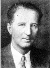
George Sterling (W1AE/W3DF). FCC commissioner in 1940, he organized and guided RID during the war. Source: National Assoc. of Broadcasters, 1948
The man behind the formation of the NDO was George Sterling. To call Sterling an early adopter of amateur radio would be an understatement. He plunged into radio as a hobby in 1908 at the tender age of 14, just a few years after Marconi and others demonstrated the potential of radio. He was licensed immediately after the passage of the Radio Act of 1927, callsign 1AE (later W1AE), and continued to experiment with spark gap stations. When the United States entered World War I, Sterling served for 19 months in France as an instructor in the Signal Corps, later organizing and operating the Corps’ first radio intelligence unit to locate enemy positions based on their radio transmissions.
After a brief post-war stint as a wireless operator in the Merchant Marine, Sterling returned to the US to begin a career in the federal government with a series of radio engineering and regulatory jobs. He rose through the ranks over the 1920s and 1930s, eventually becoming Assistant Chief of the FCC Field Division in 1937, in charge of radio engineering for the entire nation. It was on the strength of his performance in that role that he was tapped to be the first — and as it would turn out, only — chief of the NDO, which was quickly raised to the level of a new division within the FCC and renamed the Radio Intelligence Division.
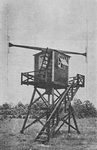
To adequately protect the homeland, the RID needed a truly national footprint. Detecting shortwave transmissions is simple enough; any single location with enough radio equipment and a suitable antenna could catch most transmissions originating from within the US or its territories. But Sterling’s experience in France taught him that a network of listening stations would be needed to accurately triangulate on a source and provide a physical location for follow-up investigation.
The network that Sterling built would eventually comprise twelve primary stations scattered around the US and its territories, including Alaska, Hawaii, and Puerto Rico. Each primary station reported directly to RID headquarters in Washington, DC, by telephone, telegraph, or teletype. Each primary station supported up to a few dozen secondary stations, with further coastal monitoring stations set up as the war ground on and German U-boats became an increasingly common threat. The network would eventually comprise over 100 stations stretched from coast to coast and beyond, staffed by almost 900 agents.
Searching the Ether
The job of staffing these stations with skilled radio operators wasn’t easy, but Sterling knew he had a ready and willing pool to pull from: his fellow hams. Recently silenced and eager to put their skills to the test, hams signed up in droves for the RID. About 80% of the RID staff were composed of current or former amateur radio operators, including the enforcement branch of sworn officers who carried badges and guns. They were the sharp end of the spear, tasked with the “last mile” search for illicit transmitters and possible confrontation with foreign agents.
But before the fedora-sporting, Tommy-gun toting G-men could swoop in to make their arrest came the tedious process of detecting and classifying potentially illicit signals. This task was made easier by an emergency order issued on December 8, 1941, the day after the Pearl Harbor attack, forbidding all amateur radio transmissions below 56 MHz. This reduced the number of targets the RID listening stations had to sort through, but the high-frequency bands cover a lot of turf, and listening to all that spectrum at the same time required a little in-house innovation.
Today, monitoring wide swaths of the spectrum is relatively easy, but in the 1940s, it was another story. Providing this capability fell to RID engineers James Veatch and William Hoffert, who invented an aperiodic receiver that covered everything from 50 kHz to 60 MHz. Called the SSR-201, this radio used a grid-leak detector to rectify and amplify all signals picked up by the antenna. A bridge circuit connected the output of the detector to an audio amplifier, with the option to switch an audio oscillator into the circuit so that continuous wave transmissions — the spy’s operating mode of choice — could be monitored. There was also an audio-triggered relay that could start and stop an external recorder, allowing for unattended operation.
SSR-201 aperiodic receiver, used by the RID to track down clandestine transmitters. Note the “Magic Eye” indicator. Source: Steve Ellington (N4LQ)
The SSR-201 and a later variant, the K-series, were built by Kann Manufacturing, a somewhat grand name for a modest enterprise operating out of the Baltimore, Maryland, basement of Manuel Kann (W3ZK), a ham enlisted by the RID to mass produce the receiver. Working with a small team of radio hobbyists and broadcast engineers mainly working after hours, Kann Manufacturing managed to make about 200 of the all-band receivers by the end of the war, mainly for the RID but also for the Office of Strategic Services (OSS), the forerunner of the CIA, as well as the intelligence services of other allied nations.
These aperiodic receivers were fairly limited in terms of sensitivity and lacked directional capability, and so were good only for a first pass scan of a specific area for the presence of a signal. Consequently, they were often used in places where enemy transmitters were likely to operate, such as major cities near foreign embassies. This application relied on the built-in relay in the receiver to trigger a remote alarm or turn on a recorder, giving the radio its nickname: “The Watchdog.” The receivers were also often mounted in mobile patrol vehicles that would prowl likely locations for espionage, such as Army bases and seaports. Much later in the war, RID mobile units would drive through remote locations such as the woods around Oak Ridge, Tennessee, and an arid plateau in the high desert near Los Alamos, New Mexico, for reasons that would soon become all too obvious.
Radio G-Men
Adcock-type goniometer radio direction finder. The dipole array could be rotated 360 degrees from inside the shack to pinpoint a bearing to the transmitter. Source: Radio Boulevard
Once a candidate signal was detected and headquarters alerted to its frequency, characteristics, and perhaps even its contents, orders went out to the primary stations to begin triangulation. Primary stations were equipped with radio direction finding (RDF) equipment, including the Adcock-type goniometer. These were generally wooden structures elevated above the ground with a distinctive Adcock antenna on the roof of the shack. The antenna was a variation on the Adcock array using two vertical dipoles on a steerable mount. The dipoles were connected to the receiving gear in the shack 180 degrees out of phase. This produced a radiation pattern with very strong nulls broadside to the antenna, making it possible for operators to determine the precise angle to the source by rotating the antenna array until the signal is minimized. Multiple stations would report the angle to the target to headquarters, where it would be mapped out and a rough location determined by where the lines intersected.
With a rough location determined, RID mobile teams would hit the streets. RID had a fleet of mobile units based on commercial Ford and Hudson models, custom-built for undercover work. Radio gear partially filled the back seat area, power supplies filled the trunk, and a small steerable loop antenna could be deployed through the roof for radio direction finding on the go. Mobile units were also equipped with special radio sets for communicating back to their primary station, using the VHF band to avoid creating unwanted targets for the other stations to monitor.
Mobile units were generally capable of narrowing the source of a transmission down to a city block or so, but locating the people behind the transmission required legwork. Armed RID enforcement agents would set out in search of the transmitter, often aided by a device dubbed “The Snifter.” This was a field-strength meter specially built for covert operations; small enough to be pocketed and monitored through headphones styled to look like a hearing aid, the agents could use the Snifter to ferret out the spy, hopefully catching them in the act and sealing their fate.
A Job (Too) Well Done
For a hastily assembled organization, the RID was remarkably effective. Originally tasked with monitoring the entire United States and its territories, that scope very quickly expanded to include almost every country in South America, where the Nazi regime found support and encouragement. Between 1940 and 1944, the RID investigated tens of thousands, resulting in 400 unlicensed stations being silenced. Not all of these were nefarious; one unlucky teenager in Portland, Oregon, ran afoul of the RID by hooking an antenna up to a record player so he could play DJ to his girlfriend down the street. But other operations led to the capture of 200 spies, including a shipping executive who used his ships to refuel Nazi U-boats operating in the Gulf of Mexico, and the famous Dusquense Spy Ring operating on Long Island.
Thanks in large part to the technical prowess of the hams populating its ranks, the RID’s success contained the seeds of its downfall. Normally, such an important self-defense task as preventing radio espionage would fall to the Army or Navy, but neither organization had the technical expertise in 1940, nor did they have the time to learn given how woefully unprepared they were for the coming war. Both branches eventually caught up, though, and neither appreciated a bunch of civilians mucking around on their turf. Turf battles ensued, politics came into it, and by 1944, budget cuts effectively ended the RID as a standalone agency.
It appears that we’re approaching the HAL-9000 point on the AI hype curve with this report, which suggests that Anthropic’s new AI model is willing to exhibit some rather antisocial behavior to achieve its goals. According to a pre-release testing summary, Claude Opus 4 was fed some hypothetical company emails that suggested engineers were planning to replace the LLM with another product. This raised Claude’s hackles enough that the model mined the email stream for juicy personal details with which to blackmail the engineers, in an attempt to win a stay of execution. True, the salacious details of an extramarital affair were deliberately seeded into the email stream, and in most cases, it tried less extreme means to stay alive, such as cajoling senior leaders by email, but in at least 84% of the test runs, Claude eventually turned to blackmail to get its way. So we’ve got that to look forward to.
Also from the world of AI, at least tangentially, it now appears possible to doxx yourself just by making comments on YouTube videos. The open-source intelligence app is called YouTube Tools, and when provided with a user’s handle, it will develop a profile of the user based on their comments and some AI magic. We wanted to give it a try, but alas, it requires a paid subscription to use, and we’re not willing to go that far even for you, dear reader. But reports are that it can infer things like the general region in which the commenter lives and discern their cultural and social leanings. The author, LolArchiver, has a range of similar mining tools for other platforms along with reverse-lookup tools for phone and email addresses, all of which likely violate the terms of service in all kinds of ways. The accuracy of the profile is obviously going to depend greatly on how much material it has to work with, so in addition to the plenty of reasons there are to avoid reading YouTube comments, now there’s a solid reason to avoid writing them.
“Danger! Code Yellow aboard the International Space Station! All hands to emergency escape pods!” OK, maybe not, but as we teased a bit on this week’s podcast, there’s now a handy desktop app that allows you to keep track of the current level of urine in the ISS’s storage tanks. The delightfully named pISSStream, which is available only for the Apple ecosystem, taps into NASA’s telemetry stream (lol) and pulls out the current level in the tanks, because why the hell not? As unserious as the project is, it did raise an interesting discussion about how fluid levels are measured in space. So we’ll be diving into that topic (yuck) for an article soon. It’ll be our number one priority.
Looks like it’s time for another Pluto pity-party with the news of a new trans-Neptunian object that might just qualify as another dwarf planet for our solar system. Bloodlessly named 2017 OF201, the object has an extremely elongated orbit, reaching from just outside Pluto’s orbit at about 44 astronomical units at perihelion and stretching more than 1,600 AUs at aphelion, and takes 25,000 years to complete. It honestly looks more like the orbit of a comet, but with an estimated diameter of 700 km, it may join the nine other likely dwarf planets, if further observations reveal that it’s properly rounded. So not only has Pluto been demoted from legit planet, it’s now just one of potentially ten or more dwarf planets plugging around out in the deep dark. Poor Pluto.
And finally, we hope this one is a gag, but we fear that the story of a Redditor unaware that analog camera film needs to be developed rings alarmingly true. The mercifully unnamed noob recently acquired a Canon AE-1 — excellent choice; that was our first “real” camera back in the day — and ran a couple of rolls of Kodak ColorPlus 200 through it. All seemed to be going well, although we suspect the photographer reflexively pulled the camera away from their eye with each exposure to check the non-existent screen on the back of the camera; old habits die hard. But when one roll of the exposed film was fed through a 35-mm scanner, the Redditor was disappointed to see nothing. Someone offered the suggestion that developing the film might be a good idea, hopefully as gently as possible. Hats off for dipping a toe in the analog world, but the follow-through is just as important as the swing.
Near my childhood home was a small river. It wasn’t much more than a creek at the best of times, and in dry summers it would sometimes almost dry up completely. But snowmelt revived it each Spring, and the remains of tropical storms in late Summer and early Fall often transformed it into a raging torrent if only briefly before the flood waters receded and the river returned to its lazy ways.
Other than to those of us who used it as a playground, the river seemed of little consequence. But it did matter enough that a mile or so downstream was some sort of instrumentation, obviously meant to monitor the river. It was — and still is — visible from the road, a tall corrugated pipe standing next to the river, topped with a box bearing the logo of the US Geological Survey. On occasion, someone would visit and open the box to do mysterious things, which suggested the river was interesting beyond our fishing and adventuring needs.
Although I learned quite early that this device was a streamgage, and that it was part of a large network of monitoring instruments the USGS used to monitor the nation’s waterways, it wasn’t until quite recently — OK, this week — that I learned how streamgages work, or how extensive the network is. A lot of effort goes into installing and maintaining this far-flung network, and it’s worth looking at how these instruments work and their impact on everyday life.
Inventing Hydrography
First, to address the elephant in the room, “gage” is a rarely used but accepted alternative spelling of “gauge.” In general, gage tends to be used in technical contexts, which certainly seems to be the case here, as opposed to a non-technical context such as “A gauge of public opinion.” Moreover, the USGS itself uses that spelling, for interesting historical reasons that they’ve apparently had to address often enough that they wrote an FAQ on the subject. So I’ll stick with the USGS terminology in this article, even if I really don’t like it that much.
With that out of the way, the USGS has a long history of monitoring the nation’s rivers. The first streamgaging station was established in 1889 along the Rio Grande River at a railroad station in Embudo, New Mexico. Measurements were entirely manual in those days, performed by crews trained on-site in the nascent field of hydrography. Many of the tools and methods that would be used through the rest of the 19th century to measure the flow of rivers throughout the West and later the rest of the nation were invented at Embudo.
Then as now, river monitoring boils down to one critical measurement: discharge rate, or the volume of water passing a certain point in a fixed amount of time. In the US, discharge rate is measured in cubic feet per second, or cfs. The range over which discharge rate is measured can be huge, from streams that trickle a few dozen cubic feet of water every second to the over one million cfs discharge routinely measured at the mouth of the mighty Mississippi each Spring.
Measurements over such a wide dynamic range would seem to be an engineering challenge, but hydrographers have simplified the problem by cheating a little. While volumetric flow in a closed container like a pipe is relatively easy — flowmeters using paddlewheels or turbines are commonly used for such a task — direct measurement of flow rates in natural watercourses is much harder, especially in navigable rivers where such measuring instruments would pose a hazard to navigation. Instead, the USGS calculates the discharge rate indirectly using stream height, often referred to as flood stage.
Beside Still Waters
Schematic of a USGS stilling well. The water level in the well tracks the height of the stream, with a bit of lag. The height of the water column in the well is easier to read than the surface of the river. Source: USGS, public domain.
The height of a river at any given point is much easier to measure, with the bonus that the tools used for this task lend themselves to continuous measurements. Stream height is the primary data point of each streamgage in the USGS network, which uses several different techniques based on the specific requirements of each site.
A float-tape gage, with a counterweighted float attached to an encoder by a stainless steel tape. The encoder sends the height of the water column in the stilling well to the data logger. Source: USGS, public domain.
The most common is based on a stilling well. Stilling wells are vertical shafts dug into the bank adjacent to a river. The well is generally large enough for a technician to enter, and is typically lined with either concrete or steel conduit, such as the streamgage described earlier. The bottom of the shaft, which is also lined with an impervious material such as concrete, lies below the bottom of the river bed, while the height of the well is determined by the highest expected flood stage for the river. The lumen of the well is connected to the river via a pair of pipes, which terminate in the water above the surface of the riverbed. Water fills the well via these input pipes, with the level inside the well matching the level of the water in the river.
As the name implies, the stilling well performs the important job of damping any turbulence in the river, allowing for a stable column of water whose height can be easily measured. Most stilling wells measure the height of the water column with a float connected to a shaft encoder by a counterweighted stainless steel tape. Other stilling wells are measured using ultrasonic transducers, radar, or even lidar scanners located in the instrument shelter on the top of the well, which translate time-of-flight to the height of the water column.
While stilling well gages are cheap and effective, they are not without their problems. Chief among these is dealing with silt and debris. Even though intakes are placed above the bottom of the river, silt enters the stilling well and settles into the sump. This necessitates frequent maintenance, usually by flushing the sump and the intake lines using water from a flushing tank located within the stilling well. In rivers with a particularly high silt load, there may be a silt trap between the intakes and the stilling well. Essentially a concrete box with a series of vertical baffles, the silt trap allows silt to settle out of the river water before it enters the stilling well, and must be cleaned out periodically.
Bubbles, Bubbles
Bubble gages often live on pilings or other structures within the watercourse.
Making up for some of the deficiencies of the stilling well is the bubble gage, which measures river stage using gas pressure. A bubble gage typically consists of a small air pump or gas cylinders inside the instrument shelter, plumbed to a pipe that comes out below the surface of the river. As with stilling wells, the tube is fixed at a known point relative to a datum, which is the reference height for that station. The end of the pipe in the water has an orifice of known size, while the supply side has regulators and valves to control the flow of gas. River stage can be measured by sensing the gas pressure in the system, which will increase as the water column above the orifice gets higher.
Bubble gages have a distinct advantage over stilling wells in rivers with a high silt load, since the positive pressure through the orifice tends to keep silt out of the works. However, bubble gages tend to need a steady supply of electricity to power their air pump continuously, or for gages using bottled gas, frequent site visits for replenishment. Also, the pipe run to the orifice needs to be kept fairly short, meaning that bubble gage instrument shelters are often located on pilings within the river course or on bridge abutments, which can make maintenance tricky and pose a hazard to navigation.
While bubble gages and stilling wells are the two main types of gaging stations for fixed installations, the USGS also maintains a selection of temporary gaging instruments for tactical use, often for response to natural disasters. These Rapid Deployment Gages (RDGs) are compact units designed to affix to the rail of a bridge or some other structure across the river. Most RDGs use radar to sense the water level, but some use sonar.
Go With the Flow
No matter what method is used to determine the stage of a river, calculating the discharge rate is the next step. To do that, hydrographers have to head to the field and make flow measurements. By measuring the flow rates at intervals across the river, preferably as close as possible to the gaging station, the total flow through the channel at that point can be estimated, and a calibration curve relating flow rate to stage can be developed. The discharge rate can then be estimated from just the stage reading.
Flow readings are taken using a variety of tools, depending on the size of the river and the speed of the current. Current meters with bucket wheels can be lowered into a river on a pole; the flow rotates the bucket wheel and closes electrical contacts that can be counted on an electromagnetic totalizer. More recently, Acoustic Doppler Current Profilers (ADCPs) have come into use. These use ultrasound to measure the velocity of particulates in the water by their Doppler shift.
Crews can survey the entire width of a small stream by wading, from boats, or by making measurements from a convenient bridge. In some remote locations where the river is especially swift, the USGS may erect a cableway across the river, so that measurements can be taken at intervals from a cable car.
Nice work if you can get it. USGS crew making flow measurements from a cableway over the American River in California using an Acoustic Doppler Current Profiler. Source: USGS, public domain.
From Paper to Satellites
In the earliest days of streamgaging, recording data was strictly a pen-on-paper process. Station log books were updated by hydrographers for every observation, with results transmitted by mail or telegraph. Later, stations were equipped with paper chart recorders using a long-duration clockwork mechanism. The pen on the chart recorder was mechanically linked to the float in a stilling well, deflecting it as the river stage changed and leaving a record on the chart. Electrical chart recorders came next, with the position of the pen changing based on the voltage through a potentiometer linked to the float.
Chart recorders, while reliable, have the twin disadvantages of needing a site visit to retrieve the data and requiring a tedious manual transcription of the chart data to tabular form. To solve the latter problem, analog-digital recorders (ADRs) were introduced in the 1960s. These recorded stage data on paper tape as four binary-coded decimal (BCD) digits. The time of each stage reading was inferred from its position on the tape, given a known starting time and reading interval. Tapes still had to be retrieved from each station, but at least reading the data back at the office could be automated with a paper tape reader.
In the 1980s and 1990s, gaging stations were upgraded to electronic data loggers, with small solar panels and batteries where grid power wasn’t available. Data was stored locally in the logger between maintenance visits by a hydrographer, who would download the data. Alternately, gaging stations located close to public rights of way sometimes had leased telephone lines for transmitting data at intervals via modem. Later, gaging stations started sprouting cross-polarized Yagi antennas, aimed at one of the Geostationary Operational Environmental Satellites (GOES). Initially, gaging stations used one of the GOES low data rate telemetry channels with a 100 to 300 bps connection. This gave hydrologists near-real-time access to gaging data for the first time. Since 2013, all stations have been upgraded to a high data rate channel that allows up to 1,200 bps telemetry.
Currently, gage data is collected every 15 minutes normally, although the interval can be increased to every 5 minutes at times of peak flow. Data is buffered locally before a GOES uplink, which is about every hour or so, or as often as every 15 minutes in peak flow or emergencies. The uplink frequencies and intervals are very well documented on the USGS site, so you can easily pick them up with an SDR, and you can see if the creek is rising from the comfort of your own shack.
Have you heard that author Andy Weir has a new book coming out? Very exciting, we know, and according to a syndicated reading list for Summer 2025, it’s called The Last Algorithm, and it’s a tale of a programmer who discovers a dark and dangerous secret about artificial intelligence. If that seems a little out of sync with his usual space-hacking fare such as The Martian and Project Hail Mary, that’s because the book doesn’t exist, and neither do most of the other books on the list.
The list was published in a 64-page supplement that ran in major US newspapers like the Chicago Sun-Times and the Philadelphia Inquirer. The feature listed fifteen must-read books, only five of which exist, and it’s no surprise that AI is to behind the muck-up. Writer Marco Buscaglia took the blame, saying that he used an LLM to produce the list without checking the results. Nobody else in the editorial chain appears to have reviewed the list either, resulting in the hallucination getting published. Readers are understandably upset about this, but for our part, we’re just bummed that Andy doesn’t have a new book coming out.
In equally exciting but ultimately fake news, we had more than a few stories pop up in our feed about NASA’s recent discovery of urban lights on an exoplanet. AI isn’t to blame for this one, though, at least not directly. Ironically, the rumor started with a TikTok video debunking a claim of city lights on a distant planet. Social media did what social media does, though, sharing only the parts that summarized the false claim and turning a debunking into a bunking. This is why we can’t have nice things.
That wasn’t the only story about distant lights, though, with this report of unexplained signals from two nearby stars. This one is far more believable, coming as it does from retired JPL scientist Richard H. Stanton, who has been using a 30″ telescope to systematically search for optical SETI signals for the past few years. These searches led to seeing two rapid pulses of light from HD 89389, an F-type star located in the constellation Ursa Major. The star rapidly brightened, dimmed, brightened again, then returned to baseline over a fraction of second; the same pattern repeated itself about 4.4 seconds later.
Intrigued, he looked back through his observations and found a similar event from a different star, HD 217014 in Pegasus, four years previously. Interestingly, this G-type star is known to have at least one exoplanet. Stanton made the first observation in 2023, and he’s spent much of the last two years ruling out things like meteor flashes or birds passing through his field of view. More study is needed to figure out what this means, and while it’s clearly not aliens, it’s fun to imagine it could be some kind of technosignature.
And one last space story, this time with the first observation of extra-solar ice. The discovery comes from the James Webb Space Telescope, which caught the telltale signature of ice crystals in a debris ring circling HD 181327, a very young star only 155 light-years away. Water vapor had been detected plenty of times outside our solar system, but not actual ice crystals until now. The ice crystals seem to be coming from collisions between icy bodies in the debris field, an observation that has interesting implications for planetary evolution.
And finally, if like us you’re impressed anytime someone busts out a project with a six-layer PCB design, wait till you get a load of this 124-layer beast. The board comes from OKI Circuit Technologies and is intended for high-bandwidth memory for AI accelerators. The dielectric for each layer is only 125-μm thick, and the board is still only 7.6 mm thick overall. At $4,800 per square meter, it’s not likely we’ll see our friends at JLC PCB offering these anytime soon, but it’s still some pretty cool engineering.
If legend is to be believed, three disparate social forces in early 20th-century America – the temperance movement, the rise of car culture, and the Scots-Irish culture of the South – collided with unexpected results. The temperance movement managed to get Prohibition written into the Constitution, which rankled the rebellious spirit of the descendants of the Scots-Irish who settled the South. In response, some of them took to the backwoods with stills and sacks of corn, creating moonshine by the barrel for personal use and profit. And to avoid the consequences of this, they used their mechanical ingenuity to modify their Fords, Chevrolets, and Dodges to provide the speed needed to outrun the law.
Though that story may be somewhat apocryphal, at least one of those threads is still woven into the American story. The moonshiner’s hotrod morphed into NASCAR, one of the nation’s most-watched spectator sports, and informed much of the car culture of the 20th century in general. Unfortunately, that led in part to our current fossil fuel predicament and its attendant environmental consequences, which are now being addressed by replacing at least some of the gasoline we burn with the same “white lightning” those old moonshiners made. The cost-benefit analysis of ethanol as a fuel is open to debate, as is the wisdom of using food for motor fuel, but one thing’s for sure: turning corn into ethanol in industrially useful quantities isn’t easy, and it requires some Big Chemistry to get it done.
Heavy on the Starch
As with fossil fuels, manufacturing ethanol for motor fuel starts with a steady supply of an appropriate feedstock. But unlike the drilling rigs and pump jacks that pull the geochemically modified remains of half-billion-year-old phytoplankton from deep within the Earth, ethanol’s feedstock is almost entirely harvested from the vast swathes of corn that carpet the Midwest US (Other grains and even non-grain plants are used as feedstock in other parts of the world, but we’re going to stick with corn for this discussion. Also, other parts of the world refer to any grain crop as corn, but in this case, corn refers specifically to maize.)
Don’t try to eat it — you’ll break your teeth. Yellow dent corn is harvested when full of starch and hard as a rock. Credit: Marjhan Ramboyong.
The corn used for ethanol production is not the same as the corn-on-the-cob at a summer barbecue or that comes in plastic bags of frozen Niblets. Those products use sweet corn bred specifically to pack extra simple sugars and less starch into their kernels, which is harvested while the corn plant is still alive and the kernels are still tender. Field corn, on the other hand, is bred to produce as much starch as possible, and is left in the field until the stalks are dead and the kernels have converted almost all of their sugar into starch. This leaves the kernels dry and hard as a rock, and often with a dimple in their top face that gives them their other name, dent corn.
Each kernel of corn is a fruit, at least botanically, with all the genetic information needed to create a new corn plant. That’s carried in the germ of the kernel, a relatively small part of the kernel that contains the embryo, a bit of oil, and some enzymes. The bulk of the kernel is taken up by the endosperm, the energy reserve used by the embryo to germinate, and as a food source until photosynthesis kicks in. That energy reserve is mainly composed of starch, which will power the fermentation process to come.
Starch is mainly composed of two different but related polysaccharides, amylose and amylopectin. Both are polymers of the simple six-carbon sugar glucose, but with slightly different arrangements. Amylose is composed of long, straight chains of glucose molecules bound together in what’s called an α-1,4 glycosidic bond, which just means that the hydroxyl group on the first carbon of the first glucose is bound to the hydroxyl on the fourth carbon of the second glucose through an oxygen atom:
Amylose, one of the main polysaccharides in starch. The glucose subunits are connected in long, unbranched chains up to 500 or so residues long. The oxygen atom binding each glucose together comes from a reaction between the OH radicals on the 1 and 4 carbons, with one oxygen and two hydrogens leaving in the form of water.
Amylose chains can be up to about 500 or so glucose subunits long. Amylopectin, on the other hand, has shorter straight chains but also branches formed between the number one and number six carbon, an α-1,6 glycosidic bond. The branches appear about every 25 residues or so, making amylopectin much more tangled and complex than amylose. Amylopectin makes up about 75% of the starch in a kernel.
Slurry Time
Ethanol production begins with harvesting corn using combine harvesters. These massive machines cut down dozens of rows of corn at a time, separating the ears from the stalks and feeding them into a threshing drum, where the kernels are freed from the cob. Winnowing fans and sieves separate the chaff and debris from the kernels, which are stored in a tank onboard the combine until they can be transferred to a grain truck for transport to a grain bin for storage and further drying.
Corn harvest in progress. You’ve got to burn a lot of diesel to make ethanol. Credit: dvande – stock.adobe.com
Once the corn is properly dried, open-top hopper trucks or train cars transport it to the distillery. The first stop is the scale house, where the cargo is weighed and a small sample of grain is taken from deep within the hopper by a remote-controlled vacuum arm. The sample is transported directly to the scale house for a quick quality assessment, mainly based on moisture content but also the physical state of the kernels. Loads that are too wet, too dirty, or have too many fractured kernels are rejected.
Loads that pass QC are dumped through gates at the bottom of the hoppers into a pit that connects to storage silos via a series of augers and conveyors. Most ethanol plants keep a substantial stock of corn, enough to run the plant for several days in case of any supply disruption. Ethanol plants operate mainly in batch mode, with each batch taking several days to complete, so a large stock ensures the efficiency of continuous operation.
The Lakota Green Plains ethanol plant in Iowa. Ethanol plants look a lot like small petroleum refineries and share some of the same equipment. Source: MsEuphonic, CC BY-SA 3.0.
To start a batch of ethanol, corn kernels need to be milled into a fine flour. Corn is fed to a hammer mill, where large steel weights swinging on a flywheel smash the tough pericarp that protects the endosperm and the germ. The starch granules are also smashed to bits, exposing as much surface area as possible. The milled corn is then mixed with clean water to form a slurry, which can be pumped around the plant easily.
The first stop for the slurry is large cooking vats, which use steam to gently heat the mixture and break the starch into smaller chains. The heat also gelatinizes the starch, in a process that’s similar to what happens when a sauce is thickened with a corn starch slurry in the kitchen. The gelatinized starch undergoes liquefaction under heat and mildly acidic conditions, maintained by injecting sulfuric acid or ammonia as needed. These conditions begin hydrolysis of some of the α-1,4 glycosidic bonds, breaking the amylose and amylopectin chains down into shorter fragments called dextrin. An enzyme, α-amylase, is also added at this point to catalyze the α-1,4 bonds to create free glucose monomers. The α-1,6 bonds are cleaved by another enzyme, α-amyloglucosidase.
The Yeast Get Busy
The result of all this chemical and enzymatic action is a glucose-rich mixture ready for fermentation. The slurry is pumped to large reactor vessels where a combination of yeasts is added. Saccharomyces cerevisiae, or brewer’s yeast, is the most common, but other organisms can be used too. The culture is supplemented with ammonia sulfate or urea to provide the nitrogen the growing yeast requires, along with antibiotics to prevent bacterial overgrowth of the culture.
Fermentation occurs at around 30 degrees C over two to three days, while the yeast gorge themselves on the glucose-rich slurry. The glucose is transported into the yeast, where each glucose molecule is enzymatically split into two three-carbon pyruvate molecules. The pyruvates are then broken down into two molecules of acetaldehyde and two of CO2. The two acetaldehyde molecules then undergo a reduction reaction that creates two ethanol molecules. The yeast benefits from all this work by converting two molecules of ADP into two molecules of ATP, which captures the chemical energy in the glucose molecule into a form that can be used to power its metabolic processes, including making more yeast to take advantage of the bounty of glucose.
Anaerobic fermentation of one mole of glucose yields two moles of ethanol and two moles of CO2.
After the population of yeast grows to the point where they use up all the glucose, the mix in the reactors, which contains about 12-15% ethanol and is referred to as beer, is pumped into a series of three distillation towers. The beer is carefully heated to the boiling point of ethanol, 78 °C. The ethanol vapors rise through the tower to a condenser, where they change back into the liquid phase and trickle down into collecting trays lining the tower. The liquid distillate is piped to the next two towers, where the same process occurs and the distillate becomes increasingly purer. At the end of the final distillation, the mixture is about 95% pure ethanol, or 190 proof. That’s the limit of purity for fractional distillation, thanks to the tendency of water and ethanol to form an azeotrope, a mixture of two or more liquids that boils at a constant temperature. To drive off the rest of the water, the distillate is pumped into large tanks containing zeolite, a molecular sieve. The zeolite beads have pores large enough to admit water molecules, but too small to admit ethanol. The water partitions into the zeolite, leaving 99% to 100% pure (198 to 200 proof) ethanol behind. The ethanol is mixed with a denaturant, usually 5% gasoline, to make it undrinkable, and pumped into storage tanks to await shipping.
Nothing Goes to Waste
The muck at the bottom of the distillation towers, referred to as whole stillage, still has a lot of valuable material and does not go to waste. The liquid is first pumped into centrifuges to separate the remaining grain solids from the liquid. The solids, called wet distiller’s grain or WDG, go to a rotary dryer, where hot air drives off most of the remaining moisture. The final product is dried distiller’s grain with solubles, or DDGS, a high-protein product used to enrich animal feed. The liquid phase from the centrifuge is called thin stillage, which contains the valuable corn oil from the germ. That’s recovered and sold as an animal feed additive, too.
Ethanol fermentation produces mountains of DDGS, or dried distiller’s grain solubles. This valuable byproduct can account for 20% of an ethanol plant’s income. Source: Inside an Ethanol Plant (YouTube).
The final valuable product that’s recovered is the carbon dioxide. Fermentation produces a lot of CO2, about 17 pounds per bushel of feedstock. The gas is tapped off the tops of the fermentation vessels by CO2 scrubbers and run through a series of compressors and coolers, which turn it into liquid carbon dioxide. This is sold off by the tanker-full to chemical companies, food and beverage manufacturers, who use it to carbonate soft drinks, and municipal water treatment plants, where it’s used to balance the pH of wastewater.
There are currently 187 fuel ethanol plants in the United States, most of which are located in the Midwest’s corn belt, for obvious reasons. Together, these plants produced more than 16 billion gallons of ethanol in 2024. Since each bushel of corn yields about 3 gallons of ethanol, that translates to an astonishing 5 billion bushels of corn used for fuel production, or about a third of the total US corn production.
Saw what you want about the wisdom of keeping a 50-year-old space mission going, but the dozen or so people still tasked with keeping the Voyager mission running are some major studs. That’s our conclusion anyway, after reading about the latest heroics that revived a set of thrusters on Voyager 1 that had been offline for over twenty years. The engineering aspects of this feat are interesting enough, but we’re more interested in the social engineering aspects of this exploit, which The Register goes into a bit. First of all, even though both Voyagers are long past their best-by dates, they are our only interstellar assets, and likely will be for centuries to come, or perhaps forever. Sure, the rigors of space travel and the ravages of time have slowly chipped away at what these machines can so, but while they’re still operating, they’re irreplaceable assets.
That makes the fix to the thruster problem all the more ballsy, since the Voyager team couldn’t be 100% sure about the status of the primary thrusters, which were shut down back in 2004. They thought it might have been that the fuel line heaters were still good, but if they actually had gone bad, trying to switch the primary thrusters back on with frozen fuel lines could have resulted in an explosion when Voyager tried to fire them, likely ending in a loss of the spacecraft. So the decision to try this had to be a difficult one, to say the least. Add in an impending shutdown of the only DSN antenna capable of communicating with the spacecraft and a two-day communications round trip, and the pressure must have been unbearable. But they did it, and Voyager successfully navigated yet another crisis. But what we’re especially excited about is discovering a 2023 documentary about the current Voyager mission team called “It’s Quieter in the Twilight.” We know what we’ll be watching this weekend.
Speaking of space exploration, one thing you don’t want to do is send anything off into space bearing Earth microbes. That would be a Very Bad Thing, especially for missions designed to look for life anywhere else but here. But, it turns out that just building spacecraft in cleanrooms might not be enough, with the discovery of 26 novel species of bacteria growing in the cleanroom used to assemble a Mars lander. The mission in question was Phoenix, which landed on Mars in 2008 to learn more about the planet’s water. In 2007, while the lander was in the Payload Hazardous Servicing Facility at Kennedy Space Center, biosurveillance teams collected samples from the cleanroom floor. Apparently, it wasn’t very clean, with 215 bacterial strains isolated, 26 of which were novel. What’s more, genomic analysis of the new bugs suggests they have genes that make them especially tough, both in their resistance to decontamination efforts on Earth and in their ability to survive the rigors of life in space. We’re not really sure if these results say more about NASA’s cleanliness than they do about the selective pressure that an extreme environment like a cleanroom exerts on fast-growing organisms like bacteria. Either way, it doesn’t bode well for our planetary protection measures.
Closer to home but more terrifying is video from an earthquake in Myanmar that has to be seen to be believed. And even then, what’s happening in the video is hard to wrap your head around. It’s not your typical stuff-falling-off-the-shelf video; rather, the footage is from an outdoor security camera that shows the ground outside of a gate literally ripping apart during the 7.7 magnitude quake in March. The ground just past the fence settles a bit while moving away from the camera a little, but the real action is the linear motion — easily three meters in about two seconds. The motion leaves the gate and landscaping quivering but largely intact; sadly, the same can’t be said for a power pylon in the distance, which crumples as if it were made from toothpicks.
And finally, “Can it run DOOM?” has become a bit of a meme in our community, a benchmark against which hacking chops can be measured. If it has a microprocessor in it, chances are someone has tried to make it run the classic first-person shooter video game. We’ve covered dozens of these hacks before, everything from a diagnostic ultrasound machine to a custom keyboard keycap, while recent examples tend away from hardware ports to software platforms such as a PDF file, Microsoft Word, and even SQL. Honestly, we’ve lost count of the ways to DOOM, which is where Can It Run Doom? comes in handy. It lists all the unique platforms that hackers have tortured into playing the game, as well as links to source code and any relevant video proof of the exploit. Check it out the next time you get the urge to port DOOM to something cool; you wouldn’t want to go through all the work to find out it’s already been done, would you?
The world’s militaries have always been at the forefront of communications technology. From trumpets and drums to signal flags and semaphores, anything that allows a military commander to relay orders to troops in the field quickly or call for reinforcements was quickly seized upon and optimized. So once radio was invented, it’s little wonder how quickly military commanders capitalized on it for field communications.
Radiotelegraph systems began showing up as early as the First World War, but World War II was the first real radio war, with every belligerent taking full advantage of the latest radio technology. Chief among these developments was the ability of signals in the high-frequency (HF) bands to reflect off the ionosphere and propagate around the world, an important capability when prosecuting a global war.
But not long after, in the less kinetic but equally dangerous Cold War period, military planners began to see the need to move more information around than HF radio could support while still being able to do it over the horizon. What they needed was the higher bandwidth of the higher frequencies, but to somehow bend the signals around the curvature of the Earth. What they came up with was a fascinating application of practical physics: meteor burst communications.
Blame It on Shannon
In practical terms, a radio signal that can carry enough information to be useful for digital communications while still being able to propagate long distances is a bit of a paradox. You can thank Claude Shannon for that, after he developed the idea of channel capacity from the earlier work of Harry Nyquist and Ralph Hartley. The resulting Hartley-Shannon Theorem states that the bit rate of a channel in a noisy environment is directly related to the bandwidth of the channel. In other words, the more data you want to stuff down a channel, the higher the frequency needs to be.
Unfortunately, that runs afoul of the physics of ionospheric propagation. Thanks to the physics of the interaction between radio waves and the charged particles between about 50 km and 600 km above the ground, the maximum frequency that can be reflected back toward the ground is about 30 MHz, which is the upper end of the HF band. Beyond that is the very-high frequency (VHF) band from 30 MHz to 300 MHz, which has enough bandwidth for an effective data channel but to which the ionosphere is essentially transparent.
Luckily, the ionosphere isn’t the only thing capable of redirecting radio waves. Back in the 1920s, Japanese physicist Hantaro Nagaoka observed that the ionospheric propagation of shortwave radio signals would change a bit during periods of high meteoric activity. That discovery largely remained dormant until after World War II, when researchers picked up on Nagoka’s work and looked into the mechanism behind his observations.
Every day, the Earth sweeps up a huge number of meteoroids; estimates range from a million to ten billion. Most of those are very small, on the order of a few nanograms, with a few good-sized chunks in the tens of kilograms range mixed in. But the ones that end up being most interesting for communications purposes are the particles in the milligram range, in part because there are about 100 million such collisions on average every day, but also because they tend to vaporize in the E-level of the ionosphere, between 80 and 120 km above the surface. The air at that altitude is dense enough to turn the incoming cosmic debris into a long, skinny trail of ions, but thin enough that the free electrons take a while to recombine into neutral atoms. It’s a short time — anywhere between 500 milliseconds to a few seconds — but it’s long enough to be useful.
A meteor trail from the annual Perseid shower, which peaks in early August. This is probably a bit larger than the optimum for MBC, but beautiful nonetheless. Source: John Flannery, CC BY-ND 2.0.
The other aspect of meteor trails formed at these altitudes that makes them useful for communications is their relative reflectivity. The E-layer of the ionosphere normally has on the order of 107 electrons per cubic meter, a density that tends to refract radio waves below about 20 MHz. But meteor trails at this altitude can have densities as high as 1011 to 1012 electrons/m3. This makes the trails highly reflective to radio waves, especially at the higher frequencies of the VHF band.
In addition to the short-lived nature of meteor trails, daily and seasonal variations in the number of meteors complicate their utility for communications. The rotation of the Earth on its axis accounts for the diurnal variation, which tends to peak around dawn local time every day as the planet’s rotation and orbit are going in the same direction and the number of collisions increases. Seasonal variations occur because of the tilt of Earth’s axis relative to the plane of the ecliptic, where most meteoroids are concentrated. More collisions occur when the Earth’s axis is pointed in the direction of travel around the Sun, which is the second half of the year for the northern hemisphere.
Learning to Burst
Building a practical system that leverages these highly reflective but short-lived and variable mirrors in the sky isn’t easy, as shown by several post-war experimental systems. The first of these was attempted by the National Bureau of Standards in 1951. They set up a system between Cedar Rapids, Iowa, and Sterling, Virginia, a path length of about 1250 km. Originally built to study propagation phenomena such as forward scatter and sporadic E, the researchers noticed significant effects on their tests by meteor trails. This made them switch their focus to meteor trails, which caught the attention of the US Air Force. They were in the market for a four-channel continuous teletype link to their base in Thule, Greenland. They got it, but only just barely, thanks to the limited technology of the time. The NBS system also used the Iowa to Virginia system to study higher data rates by pointing highly directional rhombic antennas at each end of the connection at the same small patch of sky. They managed a whopping data rate of 3,200 bits per second with this system, but only for the second or so that a meteor trail happened to appear.
The successes and failures of the NBS system made it clear that a useful system based on meteor trails would need to operate in burst mode, to jam data through the link for as long as it existed and wait for the next one. The NBS tested a burst-mode system in 1958 that used the 50-MHz band and offered a full-duplex link at 2,400 bits per second. The system used magnetic tape loops to buffer data and transmitters at both ends of the link that operated continually to probe for a path. Whenever the receiver at one end detected a sufficiently strong probe signal from the other end, the transmitter would start sending data. The Canadians got in on the MBC action with their JANET system, which had a similar dedicated probing channel and tape buffer. In 1954 they established a full-duplex teletype link between Ottawa and Nova Scotia at 1,300 bits per second with an error rate of only 1.5%
In the late 1950s, Hughes developed a single-channel air-to-ground MBC system. This was a significant development since not only had the equipment gotten small enough to install on an airplane but also because it really refined the burst-mode technology. The ground stations in the Hughes system periodically transmitted a 100-bit interrogation signal to probe for a path to the aircraft. The receiver on the ground listened for an acknowledgement from the plane, which turned the channel around and allowed the airborne transmitter to send a 100-bit data burst. The system managed a respectable 2,400 bps data rate, but suffered greatly from ground-based interference for TV stations and automotive ignition noise.
The SHAPE of Things to Come
Supreme HQ Allied Powers Europe (SHAPE), NATO’s European headquarters in the mid-60s. The COMET meteor-bounce system kept NATO commanders in touch with member-nation HQs via teletype. Source: NATO
The first major MBC system fielded during the Cold War was the Communications by Meteor Trails system, or COMET. It was used by the North Atlantic Treaty Organization (NATO) to link its far-flung outposts in member nations with Supreme Headquarters Allied Powers Europe, or SHAPE, located in Belgium. COMET took cues from the Hughes system, especially its error detection and correction scheme. COMET was a robust and effective MBC system that provided between four and eight teletype circuits depending on daily and seasonal conditions, each handling 60 words per minute.
COMET was in continuous use from the mid-1960s until well after the official end of the Cold War. By that point, secure satellite communications were nowhere near as prohibitively expensive as they had been at the beginning of the Space Age, and MBC systems became less critical to NATO. They weren’t retired, though, and COMET actually still exists, although rebranded as “Compact Over-the-Horizon Mobile Expeditionary Terminal.” These man-portable systems don’t use MBC; rather, they use high-power UHF and microwave transmitters to scatter signals off the troposphere. A small amount of the signal is reflected back to the ground, where high-gain antennas pick up the vanishingly weak signals.
Although not directly related to Cold War communications, it’s worth noting that there was a very successful MBC system fielded in the civilian space in the United States: SNOTEL. We’ve covered this system in some depth already, but briefly, it’s a network of stations in the western part of the USA with the critical job of monitoring the snowpack. A commercial MBC system connected the solar-powered monitoring stations, often in remote and rugged locations, to two different central bases. Taking advantage of diurnal meteor variations, each morning the master station would send a polling signal out to every remote, which would then send back the previous day’s data once a return path was opened. The system could collect data from 180 remote sites in just 20 minutes. It operated successfully from the mid-1970s until just recently, when pervasive cell technology and cheap satellite modems made the system obsolete.
Did artificial intelligence just jump the shark? Maybe so, and it came from the legal world of all places, with this report of an AI-generated victim impact statement. In an apparent first, the family of an Arizona man killed in a road rage incident in 2021 used AI to bring the victim back to life to testify during the sentencing phase of his killer’s trial. The video was created by the sister and brother-in-law of the 37-year-old victim using old photos and videos, and was quite well done, despite the normal uncanny valley stuff around lip-syncing that seems to be the fatal flaw for every deep-fake video we’ve seen so far. The victim’s beard is also strangely immobile, which we found off-putting.
In the video, the victim expresses forgiveness toward his killer and addresses his family members directly, talking about things like what he would have looked like if he’d gotten the chance to grow old. That seemed incredibly inflammatory to us, but according to Arizona law, victims and their families get to say pretty much whatever they want in their impact statements. While this appears to be legal, we wouldn’t be surprised to see it appealed, since the judge tacked an extra year onto the killer’s sentence over what the prosecution sought based on the power of the AI statement. If this tactic withstands the legal tests it’ll no doubt face, we could see an entire industry built around this concept.
Last week, we warned about the impending return of Kosmos 482, a Soviet probe that was supposed to go to Venus when it was launched in 1972. It never quite chooched, though, and ended up circling the Earth for the last 53 years. The satellite made its final orbit on Saturday morning, ending up in the drink in the Indian Ocean, far from land. Alas, the faint hope that it would have a soft landing thanks to the probe’s parachute having apparently been deployed at some point in the last five decades didn’t come to pass. That’s a bit of a disappointment to space fans, who’d love to get a peek inside this priceless bit of space memorabilia. Roscosmos says they monitored the descent, so presumably they know more or less where the debris rests. Whether it’s worth an expedition to retrieve it remains to be seen.
Are we really at the point where we have to worry about counterfeit thermal paste? Apparently, yes, judging by the effort Arctic Cooling is putting into authenticity verification of its MX brand pastes. To make sure you’re getting the real deal, boxes will come with seals that rival those found on over-the-counter medications and scratch-off QR codes that can be scanned and cross-referenced to an online authentication site. We suppose it makes sense; chip counterfeiting is a very real thing, after all, and it’s probably as easy to put a random glob of goo into a syringe as it is to laser new markings onto a chip package. And Arctic compound commands a pretty penny, so the incentive is obvious. But still, something about this just bothers us.
Another very cool astrophotography shot this week, this time a breathtaking collection of galaxies. Taken from the Near Infrared camera on the James Webb Space Telescope with help from the Hubble Space Telescope and the XMM-Newton X-ray space observatory, the image shows thousands of galaxies of all shapes and sizes, along with the background X-ray glow emitted by all the clouds of superheated dust and gas between them. The stars with the characteristic six-pointed diffraction spikes are all located within our galaxy, but everything else is a galaxy. The variety is fascinating, and the scale of the image is mind-boggling. It’s galactic eye candy!
And finally, if you’ve ever wondered about what happens when a nuclear reactor melts down, you’re in luck with this interesting animagraphic on the process. It’s not a detailed 3D render of any particular nuclear power plant and doesn’t have a specific meltdown event in mind, although it does mention both Chernobyl and Fukushima. Rather, it’s a general look at pressurized water reactors and what can go wrong when the cooling water stops flowing. It also touches on potentially safer designs with passive safety systems that rely on natural convection to keep cooling water circulating in the event of disaster, along with gravity-fed deluge systems to cool the containment vessel if things get out of hand. It’s a good overview of how reactors work and where they can go wrong. Enjoy.
Not too long ago, I was searching for ideas for the next installment of the “Big Chemistry” series when I found an article that discussed the world’s most-produced chemicals. It was an interesting article, right up my alley, and helpfully contained a top-ten list that I could use as a crib sheet for future articles, at least for the ones I hadn’t covered already, like the Haber-Bosch process for ammonia.
Number one on the list surprised me, though: sulfuric acid. The article stated that it was far and away the most produced chemical in the world, with 36 million tons produced every year in the United States alone, out of something like 265 million tons a year globally. It’s used in a vast number of industrial processes, and pretty much everywhere you need something cleaned or dissolved or oxidized, you’ll find sulfuric acid.
Staggering numbers, to be sure, but is it really the most produced chemical on Earth? I’d argue not by a long shot, when there’s a chemical that we make 4.4 billion tons of every year: Portland cement. It might not seem like a chemical in the traditional sense of the word, but once you get a look at what it takes to make the stuff, how finely tuned it can be for specific uses, and how when mixed with sand, gravel, and water it becomes the stuff that holds our world together, you might agree that cement and concrete fit the bill of “Big Chemistry.”
Rock Glue
To kick things off, it might be helpful to define some basic terms. Despite the tendency to use them as synonyms among laypeople, “cement” and “concrete” are entirely different things. Concrete is the finished building material of which cement is only one part, albeit a critical part. Cement is, for lack of a better term, the glue that binds gravel and sand together into a coherent mass, allowing it to be used as a building material.
What did the Romans ever do for us? The concrete dome of the Pantheon is still standing after 2,000 years. Source: Image by Sean O’Neill from Flickr via Monolithic Dome Institute (CC BY-ND 2.0)
It’s not entirely clear who first discovered that calcium oxide, or lime, mixed with certain silicate materials would form a binder strong enough to stick rocks together, but it certainly goes back into antiquity. The Romans get an outsized but well-deserved portion of the credit thanks to their use of pozzolana, a silicate-rich volcanic ash, to make the concrete that held the aqueducts together and built such amazing structures as the dome of the Pantheon. But the use of cement in one form or another can be traced back at least to ancient Egypt, and probably beyond.
Although there are many kinds of cement, we’ll limit our discussion to Portland cement, mainly because it’s what is almost exclusively manufactured today. (The “Portland” name was a bit of branding by its inventor, Joseph Aspdin, who thought the cured product resembled the famous limestone from the Isle of Portland off the coast of Dorset in the English Channel.)
Portland cement manufacturing begins with harvesting its primary raw material, limestone. Limestone is a sedimentary rock rich in carbonates, especially calcium carbonate (CaCO3), which tends to be found in areas once covered by warm, shallow inland seas. Along with the fact that limestone forms between 20% and 25% of all sedimentary rocks on Earth, that makes limestone deposits pretty easy to find and exploit.
Cement production begins with quarrying and crushing vast amounts of limestone. Cement plants are usually built alongside the quarries that produce the limestone or even right within them, to reduce transportation costs. Crushed limestone can be moved around the plant on conveyor belts or using powerful fans to blow the crushed rock through large pipes. Smaller plants might simply move raw materials around using haul trucks and front-end loaders. Along with the other primary ingredient, clay, limestone is stored in large silos located close to the star of the show: the rotary kiln.
Turning and Burning
A rotary kiln is an enormous tube, up to seven meters in diameter and perhaps 80 m long, set on a slight angle from the horizontal by a series of supports along its length. The supports have bearings built into them that allow the whole assembly to turn slowly, hence the name. The kiln is lined with refractory materials to resist the flames of a burner set in the lower end of the tube. Exhaust gases exit the kiln from the upper end through a riser pipe, which directs the hot gas through a series of preheaters that slowly raise the temperature of the entering raw materials, known as rawmix.
The rotary kiln is the centerpiece of Portland cement production. While hard to see in this photo, the body of the kiln tilts slightly down toward the structure on the left, where the burner enters and finished clinker exits. Source: by nordroden, via Adobe Stock (licensed).
Preheating the rawmix drives off any remaining water before it enters the kiln, and begins the decomposition of limestone into lime, or calcium oxide:
The rotation of the kiln along with its slight slope results in a slow migration of rawmix down the length of the kiln and into increasingly hotter regions. Different reactions occur as the temperature increases. At the top of the kiln, the 500 °C heat decomposes the clay into silicate and aluminum oxide. Further down, as the heat reaches the 800 °C range, calcium oxide reacts with silicate to form the calcium silicate mineral known as belite:
Finally, near the bottom of the kiln, belite and calcium oxide react to form another calcium silicate, alite:
It’s worth noting that cement chemists have a specialized nomenclature for alite, belite, and all the other intermediary phases of Portland cement production. It’s a shorthand that looks similar to standard chemical nomenclature, and while we’re sure it makes things easier for them, it’s somewhat infuriating to outsiders. We’ll stick to standard notation here to make things simpler. It’s also important to note that the aluminates that decomposed from the clay are still present in the rawmix. Even though they’re not shown in these reactions, they’re still critical to the proper curing of the cement.
Portland cement clinker. Each ball is just a couple of centimeters in diameter. Source: مرتضا, Public domain
The final section of the kiln is the hottest, at 1,500 °C. The extreme heat causes the material to sinter, a physical change that partially melts the particles and adheres them together into small, gray lumps called clinker. When the clinker pellets drop from the bottom of the kiln, they are still incandescently hot. Blasts of air that rapidly bring the clinker down to around 100 °C. The exhaust from the clinker cooler joins the kiln exhaust and helps preheat the incoming rawmix charge, while the cooled clinker is mixed with a small amount of gypsum and ground in a ball mill. The fine gray powder is either bagged or piped into bulk containers for shipment by road, rail, or bulk cargo ship.
The Cure
Most cement is shipped to concrete plants, which tend to be much more widely distributed than cement plants due to the perishable nature of the product they produce. True, both plants rely on nearby deposits of easily accessible rock, but where cement requires limestone, the gravel and sand that go into concrete can come from a wide variety of rock types.
Concrete plants quarry massive amounts of rock, crush it to specifications, and stockpile the material until needed. Orders for concrete are fulfilled by mixing gravel and sand in the proper proportions in a mixer housed in a batch house, which is elevated above the ground to allow space for mixer trucks to drive underneath. The batch house operators mix aggregate, sand, and any other admixtures the customer might require, such as plasticizers, retarders, accelerants, or reinforcers like chopped fiberglass, before adding the prescribed amount of cement from storage silos. Water may or may not be added to the mix at this point. If the distance from the concrete plant to the job site is far enough, it may make sense to load the dry mix into the mixer truck and add the water later. But once the water goes into the mix, the clock starts ticking, because the cement begins to cure.
Cement curing is a complex process involving the calcium silicates (alite and belite) in the cement, as well as the aluminate phases. Overall, the calcium silicates are hydrated by the water into a gel-like substance of calcium oxide and silicate. For alite, the reaction is:
Scanning electron micrograph of cured Portland cement, showing needle-like ettringite and plate-like calcium oxide. Source: US Department of Transportation, Public domain
At the same time, the aluminate phases in the cement are being hydrated and interacting with the gypsum, which prevents early setting by forming a mineral known as ettringite. Without the needle-like ettringite crystals, aluminate ions would adsorb onto alite and block it from hydrating, which would quickly reduce the plasticity of the mix. Ideally, the ettringite crystals interlock with the calcium silicate gel, which binds to the surface of the sand and gravel and locks it into a solid.
Depending on which adjuvants were added to the mix, most concretes begin to lose workability within a few hours of rehydration. Initial curing is generally complete within about 24 hours, but the curing process continues long after the material has solidified. Concrete in this state is referred to as “green,” and continues to gain strength over a period of weeks or even months.
By now, you’ve probably heard about Kosmos 482, a Soviet probe destined for Venus in 1972 that fell a bit short of the mark and stayed in Earth orbit for the last 53 years. Soon enough, though, the lander will make its fiery return; exactly where and when remain a mystery, but it should be sometime in the coming week. We talked about the return of Kosmos briefly on this week’s podcast and even joked a bit about how cool it would be if the parachute that would have been used for the descent to Venus had somehow deployed over its half-century in space. We might have been onto something, as astrophotographer Ralf Vanderburgh has taken some pictures of the spacecraft that seem to show a structure connected to and trailing behind it. The chute is probably in pretty bad shape after 50 years of UV torture, but how cool is that?
Parachute or not, chances are good that the 495-kilogram spacecraft, built to not only land on Venus but to survive the heat, pressure, and corrosive effects of the hellish planet’s atmosphere, will at least partially survive reentry into Earth’s more welcoming environs. That’s a good news, bad news thing: good news that we might be able to recover a priceless artifact of late-Cold War space technology, bad news to anyone on the surface near where this thing lands. If Kosmos 482 does manage to do some damage, it won’t be the first time. Shortly after launch, pieces of titanium rained down on New Zealand after the probe’s booster failed to send it on its way to Venus, damaging crops and starting some fires. The Soviets, ever secretive about their space exploits until they could claim complete success, disavowed the debris and denied responsibility for it. That made the farmers whose fields they fell in the rightful owners, which is also pretty cool. We doubt that the long-lost Kosmos lander will get the same treatment, but it would be nice if it did.
Also of note in the news this week is a brief clip of a Unitree humanoid robot going absolutely ham during a demonstration — demo-hell, amiright? Potential danger to the nearby engineers notwithstanding, the footage is pretty hilarious. The demo, with a robot hanging from a hoist in a crowded lab, starts out calmly enough, but goes downhill quickly as the robot starts flailing its arms around. We’d say the movements were uncontrolled, but there are points where the robot really seems to be chasing the engineer and taking deliberate swipes at the poor guy, who was probably just trying to get to the e-stop switch. We know that’s probably just the anthropomorphization talking, but it sure looks like the bot had a beef to settle. You be the judge.
Also from China comes a report of “reverse ATMs” that accept gold and turn it into cash on the spot (apologies for yet another social media link, but that’s where the stories are these days). The machine shown has a hopper into which customers can load their unwanted jewelry, after which it is reportedly melted down and assayed for purity. The funds are then directly credited to the customer’s account electronically. We’re not sure we fully believe this — thinking about the various failure modes of one of those fresh-brewed coffee machines, we shudder to think about the consequences of a machine with a 1,000°C furnace built into it. We also can’t help but wonder how the machine assays the scrap gold — X-ray fluorescence? Ramann spectroscopy? Also, what happens to the unlucky customer who puts some jewelry in that they thought was real gold, only to be told by the machine that it wasn’t? Do they just get their stuff back as a molten blob? The mind boggles.
And finally, the European Space Agency has released a stunning new image of the Sun. Captured by their Solar Orbiter spacecraft in March from about 77 million kilometers away, the mosaic is composed of about 200 images from the Extreme Ultraviolet Imager. The Sun was looking particularly good that day, with filaments, active regions, prominences, and coronal loops in evidence, along with the ethereal beauty of the Sun’s atmosphere. The image is said to be the most detailed view of the Sun yet taken, and needs to be seen in full resolution to be appreciated. Click on the image below and zoom to your heart’s content.